SAEM in nlmixr2: robust stochastic-approximation EM

nlmixr

SAEM (`est = "saem"`): the robust stochastic EM

est = "saem" is nlmixr2’s Stochastic Approximation Expectation-Maximization method (Kuhn & Lavielle 2005), and – with focei – one of the two workhorses. Where the conditional-estimation ladder approximates the marginal likelihood analytically (a Laplace-type expansion), SAEM sidesteps that approximation entirely: it draws the random effects with MCMC and updates the population parameters by stochastic approximation. That makes it exceptionally robust – it keeps working on nonlinear models, mixtures, and awkward posteriors where a Laplace approximation is unreliable or an optimizer gets stuck.

This article leads with a worked example; the algorithm follows.

Worked example: watch it converge, and check it against FOCEI

The theophylline model, one compartment, between-subject variability on ka, cl and v:

library(nlmixr2)

theoModel <- function() {
  ini({
    tka <- 0.45; tcl <- 1; tv <- 3.45
    eta.ka ~ 0.6; eta.cl ~ 0.3; eta.v ~ 0.1
    add.sd <- 0.7
  })
  model({
    ka <- exp(tka + eta.ka)
    cl <- exp(tcl + eta.cl)
    v  <- exp(tv  + eta.v)
    d/dt(depot)  <- -ka * depot
    d/dt(center) <-  ka * depot - cl / v * center
    cp <- center / v
    cp ~ add(add.sd)
  })
}

saemControl() sets the two phases of the run explicitly: nBurn exploratory iterations (a constant, large stochastic step that lets the chain roam), then nEm convergence iterations (a shrinking Robbins-Monro step that averages the noise away):

fitSaem  := nlmixr2(theoModel, nlmixr2data::theo_sd, est = "saem",
                    control = saemControl(nBurn = 250L, nEm = 350L, print = 0L))
fitFocei := nlmixr2(theoModel, nlmixr2data::theo_sd, est = "focei",
                    control = foceiControl(print = 0L))

The signature SAEM convergence trajectory

The whole parameter history is stored in the fit. Plotting it shows SAEM’s two phases unmistakably – noisy exploration up to nBurn, then a smooth settle:

library(ggplot2)

nBurn <- 250
ph <- fitSaem$parHistData
keep <- c("tka", "tcl", "tv", "V(eta.ka)", "V(eta.cl)", "V(eta.v)", "add.sd")
long <- do.call(rbind, lapply(keep, function(p)
  data.frame(iter = ph$iter, parameter = p, value = ph[[p]])))
long$parameter <- factor(long$parameter, levels = keep)

ggplot(long, aes(iter, value)) +
  geom_vline(xintercept = nBurn, linetype = 2, colour = "tomato") +
  geom_line(linewidth = 0.4, colour = "steelblue") +
  facet_wrap(~ parameter, scales = "free_y") +
  labs(x = "iteration", y = NULL,
       title = "SAEM: stochastic exploration (left of the line), then convergence") +
  theme_bw()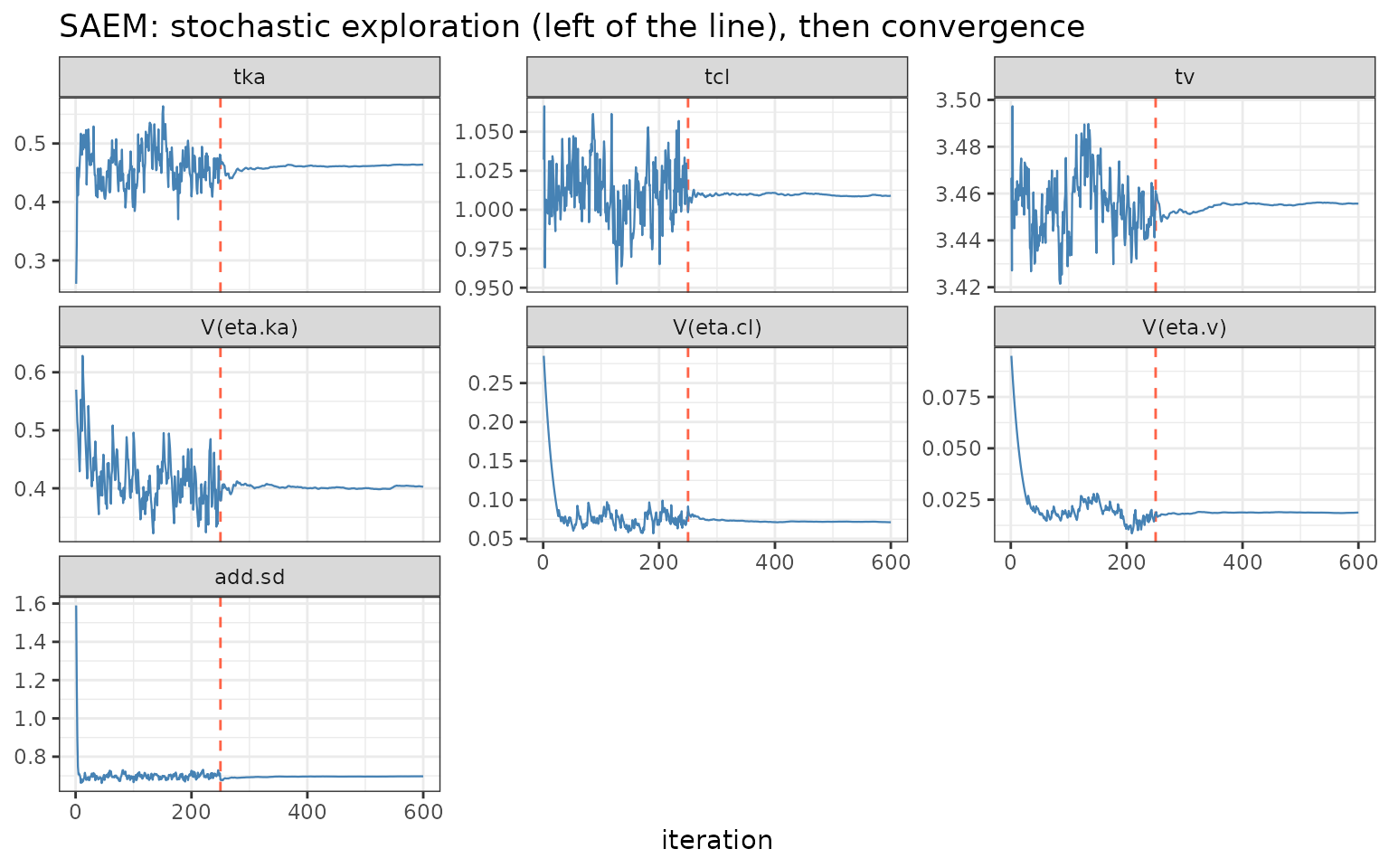

Left of the red line the chain explores; right of it the decreasing step size drives it to the maximum-likelihood estimate. Watching this plot is the standard way to judge SAEM convergence – if the right-hand phase has not flattened, increase nEm.

It agrees with FOCEI

On a model where FOCEI’s Laplace approximation is accurate, SAEM lands in the same place – a reassuring cross-check from a completely different estimation principle:

round(rbind(FOCEI = fitFocei$theta, SAEM = fitSaem$theta), 3)
#>         tka   tcl    tv add.sd
#> FOCEI 0.463 1.012 3.460  0.694
#> SAEM  0.464 1.009 3.456  0.697
round(rbind(FOCEI = diag(fitFocei$omega), SAEM = diag(fitSaem$omega)), 3)
#>       eta.ka eta.cl eta.v
#> FOCEI  0.400  0.069 0.019
#> SAEM   0.403  0.071 0.019

A note on the objective: SAEM’s reported -2LL is computed by a separate likelihood step (importance sampling or Gaussian quadrature) with its own constant convention, so it is not directly comparable to a FOCEI or IMP objective. Compare SAEM to SAEM.

When to choose SAEM

Reach for saem when:

the model is strongly nonlinear or the individual posteriors are non-Gaussian, so a Laplace approximation (FOCEI/laplace) may be biased – SAEM makes no such approximation;
you are fitting a mixture model (distinct subpopulations); SAEM’s MCMC E-step handles the discrete mixture indicator naturally (see the mixture-models article);
an optimizer-based method fails to converge or is sensitive to starting values – SAEM’s stochastic exploration is far less prone to getting stuck;
you have many random effects or a complex covariance structure, where the robustness of the stochastic E-step pays off.

Prefer FOCEI when the model is close to linear and you want the fastest deterministic fit with an immediately comparable objective function; use the importance-sampling EM family when you specifically need a Monte-Carlo exact marginal likelihood (SAEM does not return one directly).

How SAEM works

SAEM is an EM algorithm whose E-step is done by simulation. Each iteration:

Simulation (stochastic E-step). Rather than integrate the random effects out analytically, SAEM samples them: a Metropolis-Hastings chain draws each subject’s eta from its conditional posterior p(eta | y_i, theta) at the current parameters. No linearization, no Laplace expansion.
Stochastic approximation. The complete-data sufficient statistics are updated as a running average with step size gamma_k. During burn-in (k <= nBurn) gamma_k = 1, so the statistics track the exploring chain; during convergence (k > nBurn) gamma_k decreases (Robbins-Monro), averaging out the Monte-Carlo noise so the estimates settle.
Maximization (M-step). Given the (approximate) sufficient statistics, the population parameters – typical values, Omega, residual error – have closed-form updates for mu-referenced models, which is what makes each iteration cheap.

Two practical consequences: the objective is not produced by the algorithm itself (nlmixr2 computes the -2LL afterward, by importance sampling or Gaussian quadrature), and the fit is stochastic – reproducible for a fixed seed, but you should confirm convergence from the trajectory rather than from a single objective value.

The same idea, a different implementation: babelmixr2 `saemix`

babelmixr2 exposes a second SAEM through est = "saemix", which runs the saemix R package (Comets, Lavielle & Kuhn) on the same nlmixr2 model and wraps the result as an nlmixr2 fit. Because both implement the same algorithm, saemix is a natural independent cross-check of an est = "saem" run:

library(babelmixr2)
fitSaemix <- nlmixr2(theoModel, nlmixr2data::theo_sd, est = "saemix",
                     control = saemixControl())

How it relates to the other methods

	FOCEI / laplace / agq	SAEM	imp / impmap / qrpem
Marginal likelihood	Analytic approximation	Not used during fitting (MCMC E-step)	Monte-Carlo (near-exact)
E-step	Conditional mode	MCMC sampling	Importance sampling
Robustness on hard/multimodal models	Lower	High	Medium
Objective for model comparison	Directly	Separate step, own constant	Directly (matches NONMEM IMP)
External equivalents	NONMEM FOCE(I); Phoenix FOCE	NONMEM SAEM; Monolix; saemix	NONMEM IMP/IMPMAP; Phoenix QRPEM

est = "saem" corresponds to the SAEM in NONMEM (METHOD=SAEM), Monolix (whose engine is SAEM), and the saemix package – all the same Kuhn-Lavielle algorithm. It is the robust, approximation-free member of the nlmixr2 estimation family, complementary to FOCEI’s speed and the importance-sampling family’s exact likelihood.

References

Kuhn E, Lavielle M. Maximum likelihood estimation in nonlinear mixed effects models. Computational Statistics & Data Analysis, 2005.
Delyon B, Lavielle M, Moulines E. Convergence of a stochastic approximation version of the EM algorithm. Annals of Statistics, 1999.
Comets E, Lavielle M, Kuhn E. saemix: an R version of the SAEM algorithm. (the saemix package, exposed via babelmixr2).

2026-09-15

SAEM (est = "saem"): the robust stochastic EM