Delay differential equations (DDEs) in nlmixr2

library(nlmixr2)
library(ggplot2)

Most PKPD models say that the rate of change of a system depends on where the system is now:

$$\frac{d}{dt}x(t) = f(t, x(t)), \qquad x(0) = x_0$$

Biology often disagrees. A cell that is dying today was marked for death by a drug concentration it saw several days ago; a platelet entering the circulation today was produced a week ago. In these systems the rate of change depends on where the system was, which is a delay differential equation (DDE):

$$\frac{d}{dt}x(t) = f\big(t,\, x(t),\, x(t - T)\big), \qquad x(t) = x_0(t) \;\;\text{for}\; -T \le t \le 0$$

Koch, Krzyzanski, Pérez-Ruixo and Schropp¹ give a tutorial on these models and the two features that distinguish them from ODEs:

1. the mechanism depends on the delayed state $x(t-T)$, so there is an explicit delay parameter $T$ that can be estimated; and
2. a DDE needs a past $x_0(t)$ on $[-T, 0]$ — a whole function, not just an initial value — because the system starts by reading history that predates $t = 0$.

rxode2 (and therefore nlmixr2) expresses both directly:

Concept	Syntax
the delayed state $x(t-T)$	delay(x, T)
a non-constant past $x_0(t)$	past(x, T) <- expr

Without a past() statement the pre-history is the state’s initial condition, held constant — which is what most models want. past() is for the models that need more, and we get to one below.

This article works two of Koch’s examples end to end: we simulate each model from the paper’s own published parameter values, then estimate it back — using the same kind of estimation the original article used for each. Example 2 was an individual fit in Berkeley Madonna, so we use a derivative-free optimizer (est="bobyqa"); Example 6 was a population fit in Monolix, so we use est="ifoceif" (FOCEi with a mu-referenced IRLS inner problem and the analytic Almquist outer gradient). In both, the delay is recovered from the data.

Why bother? Delays versus transit compartments

The usual way to put a delay into an ODE model is a chain of transit compartments. That is a genuinely different model: a transit chain spreads the delay out (each molecule takes a random, gamma-distributed time to traverse it), whereas a lifespan model says every cell lives exactly $T$ days. When the underlying biology really is a lifespan, the DDE is both more faithful and much smaller — two equations instead of $n$.

Example 2: lifespan-based tumour growth

Simeoni’s xenograft model routes drug-damaged cells through a chain of transit compartments $d_1 \ldots d_n$ before they die. Koch’s Example 2 rewrites it so that damaged cells instead die after an exact lifespan $T_d$. The whole chain collapses into one equation whose outflow is its own inflow, delayed:

$$\frac{d}{dt}p(t) = g\big(k_0,k_1,p(t),d(t)\big) - k_{pot}\,c(t)\,p(t), \qquad p(0)=w_0$$$$\frac{d}{dt}d(t) = \underbrace{k_{pot}\,c(t)\,p(t)}_{\text{damaged now}} - \underbrace{k_{pot}\,c(t-T_d)\,p(t-T_d)}_{\text{damaged } T_d \text{ ago, now dead}}, \qquad d(0)=0$$

with total tumour weight $w(t) = p(t) + d(t)$ and growth

$$g(k_0,k_1,p,d) = \frac{2k_0k_1p^2}{(k_1 + 2k_0p)(p+d)}$$

Here the past is constant and zero: no drug is given before the tumour is inoculated, so $k_{pot}c(t)p(t) = 0$ for $-T_d \le t \le 0$. delay() alone covers it — the default constant pre-history is exactly right.

The parameters below are the paper’s own Berkeley Madonna values (Appendix 2): a 100 mg dose daily on days 12–16.

ex2 <- rxode2({
  ka <- 103.96 * 24; ke <- 0.1052 * 24; V <- 2.7882
  l0 <- 0.195; l1 <- 0.245; w0 <- 0.010
  kpot <- 0.007; tau <- 3.61
  d/dt(x1) <- -ka * x1                      # depot
  d/dt(x2) <- ka * x1 - ke * x2             # central
  c    <- x2 / V
  cdel <- delay(x2, tau) / V                # concentration tau days ago
  ## untreated control tumour, for reference
  d/dt(x3) <- (2 * l0 * l1 * x3) / (l1 + 2 * l0 * x3)
  ## proliferating cells
  d/dt(x4) <- (2 * l0 * l1 * x4^2) / ((l1 + 2 * l0 * x4) * (x4 + x5)) - kpot * c * x4
  ## apoptotic cells: damaged now, minus damaged exactly tau days ago
  d/dt(x5) <- kpot * c * x4 - kpot * cdel * delay(x4, tau)
  x3(0) <- w0; x4(0) <- w0; x5(0) <- 0
  w <- x4 + x5                              # total tumour weight
})

A DDE has to interpolate its own history, so the solver must retain it: pass dense=TRUE (and a suitable method) when solving by hand.

ev2 <- et(seq(0, 30, by = 0.25))
for (td in 12:16) ev2 <- et(ev2, amt = 300, cmt = "x1", time = td)

s2 <- rxSolve(ex2, ev2, method = "dop853", dense = TRUE, atol = 1e-10, rtol = 1e-10)

ggplot(s2, aes(time)) +
  geom_line(aes(y = x3, colour = "untreated control")) +
  geom_line(aes(y = w, colour = "treated")) +
  annotate("rect", xmin = 12, xmax = 16, ymin = -Inf, ymax = Inf, alpha = 0.1) +
  labs(x = "time (days)", y = "tumour weight (g)", colour = NULL,
       title = "Koch Example 2: lifespan-based tumour growth",
       subtitle = "shaded band = dosing days 12-16") +
  theme_bw() + theme(legend.position = "top")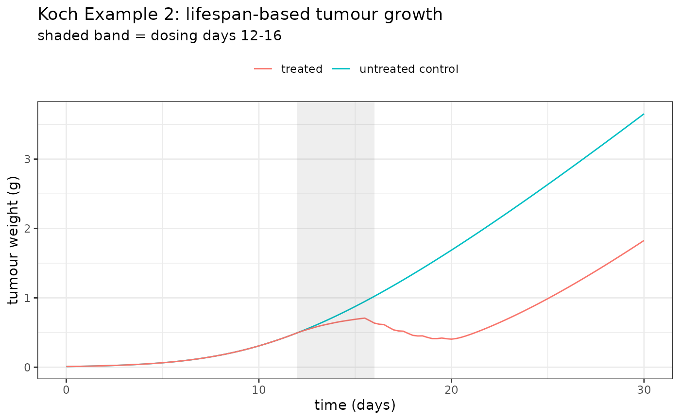

Simulating a population

To show the delay can be recovered, we simulate 24 mice with between-subject variability on the drug potency kpot and on the apoptotic lifespan tau itself, and observe tumour weight with additive error.

sim2 <- rxode2({
  ka <- 103.96 * 24; ke <- 0.1052 * 24; V <- 2.7882
  l0 <- 0.195; l1 <- 0.245; w0 <- 0.010
  kpot <- 0.007 * exp(eta.kpot)
  tau  <- 3.61 * exp(eta.tau)
  d/dt(x1) <- -ka * x1
  d/dt(x2) <- ka * x1 - ke * x2
  c    <- x2 / V
  cdel <- delay(x2, tau) / V
  d/dt(x4) <- (2 * l0 * l1 * x4^2) / ((l1 + 2 * l0 * x4) * (x4 + x5)) - kpot * c * x4
  d/dt(x5) <- kpot * c * x4 - kpot * cdel * delay(x4, tau)
  x4(0) <- w0; x5(0) <- 0
  w <- x4 + x5
})

set.seed(101)
obst <- c(0, 3, 6, 9, 12, 14, 16, 18, 20, 22, 24, 26, 28, 30)
N <- 16
dose <- 300     # a strong drug effect makes the delayed apoptotic removal --
ev <- et(obst)  # and hence the lifespan -- observable in the tumour weight
for (td in 12:16) ev <- et(ev, amt = dose, cmt = "x1", time = td)

rows <- list()
for (i in 1:N) {
  p <- c(eta.kpot = rnorm(1, 0, sqrt(0.04)), eta.tau = rnorm(1, 0, sqrt(0.02)))
  s <- rxSolve(sim2, params = p, ev, method = "dop853", dense = TRUE,
               returnType = "data.frame", atol = 1e-8, rtol = 1e-8)
  s <- s[s$time %in% obst, ]
  dv <- s$w + rnorm(nrow(s), 0, 0.02); dv[dv <= 0] <- 1e-3
  rows[[i]] <- data.frame(ID = i, TIME = s$time, DV = dv, AMT = 0, EVID = 0, CMT = "x4")
}
obs <- do.call(rbind, rows)
dos <- do.call(rbind, lapply(1:N, function(i)
  data.frame(ID = i, TIME = 12:16, DV = NA_real_, AMT = dose, EVID = 1, CMT = "x1")))
dat2 <- rbind(obs, dos)
dat2 <- dat2[order(dat2$ID, dat2$TIME, -dat2$EVID), ]
head(dat2)
#>     ID TIME         DV AMT EVID CMT
#> 1    1    0 0.00100000   0    0  x4
#> 2    1    3 0.02254589   0    0  x4
#> 3    1    6 0.09352435   0    0  x4
#> 4    1    9 0.24500364   0    0  x4
#> 225  1   12         NA 300    1  x1
#> 5    1   12 0.52642045   0    0  x4

Estimating it back

Koch et al. fit this example in Berkeley Madonna as an individual model — no random effects — and estimated the lifespan Td directly from the data (their Table 1). We do the same: a single-subject / naive-pooled fit estimating the drug potency kpot and the apoptotic lifespan tau (the delay).

The choice of optimizer matters here, and it is worth understanding why. The delay parameter sits inside a product of two delayed states, delay(x2, tau) * delay(x4, tau), and the PK is stiff. A parameter like that is awkward for a gradient-based optimizer: the model’s exact derivative with respect to the delay time is expensive, and a finite-difference gradient is noisy because moving tau slides the interpolated history. So we use est="bobyqa" — Powell’s derivative-free bounded optimizer, which only ever evaluates the objective and never differentiates it. That is exactly the kind of optimizer Berkeley Madonna uses, and it walks straight to the minimum.

mod2 <- function() {
  ini({
    tkpot <- c(log(0.002), log(0.006), log(0.02))   # bounded; truth 0.007
    ttau  <- c(log(1.5),   log(3.0),   log(6.0))    # bounded; Td, truth 3.61
    add.err <- c(0.001, 0.02, 0.2)
  })
  model({
    ka <- 103.96 * 24; ke <- 0.1052 * 24; V <- 2.7882
    l0 <- 0.195; l1 <- 0.245; w0 <- 0.010
    kpot <- exp(tkpot)
    tau  <- exp(ttau)
    d/dt(x1) <- -ka * x1
    d/dt(x2) <- ka * x1 - ke * x2
    c    <- x2 / V
    cdel <- delay(x2, tau) / V
    d/dt(x4) <- (2 * l0 * l1 * x4^2) / ((l1 + 2 * l0 * x4) * (x4 + x5)) - kpot * c * x4
    d/dt(x5) <- kpot * c * x4 - kpot * cdel * delay(x4, tau)
    x4(0) <- w0; x5(0) <- 0
    w <- x4 + x5
    w ~ add(add.err)
  })
}

optExpression=FALSE turns off common-subexpression optimization: a delay() term has to be regenerated together with the d/dt() of the state it delays, which defeats the optimizer’s model-splitting on a DDE and makes assembly slow. Turning it off skips that; the model solves fine without it.

fit2 := nlmixr2(mod2, dat2, est = "bobyqa",
                control = bobyqaControl(optExpression = FALSE))
fit2

$$\begin{align*} {ka} & = {103.96} {\times} {24} \\ {ke} & = {0.1052} {\times} {24} \\ {V} & = {2.7882} \\ {l0} & = {0.195} \\ {l1} & = {0.245} \\ {w0} & = {0.01} \\ {kpot} & = \exp\left({tkpot}\right) \\ {tau} & = \exp\left({ttau}\right) \\ \frac{d \: x1}{dt} & = -{ka} {\times} {x1} \\ \frac{d \: x2}{dt} & = {ka} {\times} {x1}-{ke} {\times} {x2} \\ {c} & = \frac{{x2}}{{V}} \\ {cdel} & = \frac{delay({x2}, {tau})}{{V}} \\ \frac{d \: x4}{dt} & = \frac{\left({2} {\times} {l0} {\times} {l1} {\times} {{x4}}^{{2}}\right)}{\left(\left({l1}+{2} {\times} {l0} {\times} {x4}\right) {\times} \left({x4}+{x5}\right)\right)}-{kpot} {\times} {c} {\times} {x4} \\ \frac{d \: x5}{dt} & = {kpot} {\times} {c} {\times} {x4}-{kpot} {\times} {cdel} {\times} delay({x4}, {tau}) \\ x4({0}) & = {w0} \\ x5({0}) & = {0} \\ {w} & = {x4}+{x5} \\ {w} & \sim add({add.err}) \end{align*}$$

truth2 <- c(kpot = 0.007, tau = 3.61)
est2 <- exp(fixef(fit2)[c("tkpot", "ttau")])
data.frame(parameter = names(truth2),
           truth = truth2,
           estimate = round(est2, 4),
           ratio = round(est2 / truth2, 3),
           row.names = NULL)
#>   parameter truth estimate ratio
#> 1      kpot 0.007   0.0068 0.975
#> 2       tau 3.610   3.7153 1.029

The apoptotic lifespan tau is recovered close to its true 3.61 days — the delay is estimated directly from the tumour-weight data, exactly as in the original article.

Example 6: a model whose past is not constant

Example 2 got away with the default pre-history because nothing happened before $t=0$. Koch’s Example 6 does not.

In collagen-induced arthritic mice, arthritis has an induction phase with no measurements, followed by a development phase where data collection starts. The cytokine GM-CSF is already being over-produced during induction, so at $t = 0$ the system is mid-flight: its history is a growing exponential, not a constant. The model (a total arthritic score $R_1$, and a strongly delayed ankylosis score $R_2$) reads

$$\frac{d}{dt}G(t) = k_3 - \frac{k_1}{k_2}\big(1 - e^{-k_2 t}\big)G(t) - \frac{E_{max}c(t)}{EC_{50}+c(t)}G(t), \qquad \boxed{G(t) = a e^{bt} \;\text{for}\; -T \le t \le 0}$$$$\frac{d}{dt}I(t) = k_4 G(t) - k_4 G(t-T), \qquad I(0)=I_0$$$$\frac{d}{dt}D(t) = k_4 G(t-T) - k_5 D(t), \qquad D(0)=0$$$$R_1(t) = I(t) + D(t) \quad\text{(TAS)}, \qquad R_2(t) = D(t) \quad\text{(AKS)}$$

That boxed line is the whole point. $D$ is driven by $G(t-T)$ with $T \approx 13$ days, so for the first two weeks the ankylosis score is driven entirely by cytokine history that predates the study. Get the past wrong and the entire induction/early-response phase is wrong.

The paper implements this in MONOLIX, where the delayed state’s initial condition is written as an expression in t (y1_0 = a*exp(b*t)). rxode2 says the same thing with past():

ex6 <- rxode2({
  k  <- 0.184; V <- 0.039
  k1 <- 0.535; k2 <- 0.352; k3 <- 5
  k4 <- 0.122; k5 <- 0.126
  Emax <- 1; EC50 <- 44.3
  T  <- 12.8; I0 <- 2.42
  a  <- 1; b <- 0.5
  d/dt(Ac) <- -k * Ac
  c   <- Ac / V
  eff <- (Emax * c) / (EC50 + c)
  G(0) <- a                     # continuity: a*exp(b*0) = a
  d/dt(G) <- k3 - eff * G - (k1 / k2) * (1 - exp(-k2 * t)) * G
  past(G, T) <- a * exp(b * t)  # <- the induction-phase history, on [-T, 0]
  I(0) <- I0
  d/dt(I) <- k4 * G - k4 * delay(G, T)
  D(0) <- 0
  d/dt(D) <- k4 * delay(G, T) - k5 * D
  TAS <- I + D
  AKS <- D
})

Checking the past against the paper

Koch derives the model’s own closed form on $[0, T]$ (their Eqs. 85–87): while $t \le T$, the delayed cytokine is just the history evaluated at $t-T$, i.e. $G(t-T) = a\,e^{b(t-T)}$. That is an exact statement we can test.

probe <- rxode2({
  T <- 12.8; a <- 1; b <- 0.5
  k3 <- 5; k1 <- 0.535; k2 <- 0.352
  G(0) <- a
  d/dt(G) <- k3 - (k1 / k2) * (1 - exp(-k2 * t)) * G
  past(G, T) <- a * exp(b * t)
  gdel <- delay(G, T)
})
tt <- seq(0, 12.8, by = 0.1)
sp <- rxSolve(probe, et(tt), method = "dop853", dense = TRUE, atol = 1e-10, rtol = 1e-10)
max(abs(sp$gdel - 1 * exp(0.5 * (tt - 12.8))))   # vs the paper's Eq (86)/(87)
#> [1] 0

Zero — past() reproduces the published closed form exactly.

It is worth seeing what the default constant pre-history would have done here, since that is the trap this syntax exists to avoid:

ex6const <- rxode2({
  k <- 0.184; V <- 0.039; k1 <- 0.535; k2 <- 0.352; k3 <- 5
  k4 <- 0.122; k5 <- 0.126; Emax <- 1; EC50 <- 44.3
  T <- 12.8; I0 <- 2.42; a <- 1
  d/dt(Ac) <- -k * Ac
  c   <- Ac / V
  eff <- (Emax * c) / (EC50 + c)
  G(0) <- a
  d/dt(G) <- k3 - eff * G - (k1 / k2) * (1 - exp(-k2 * t)) * G
  I(0) <- I0
  d/dt(I) <- k4 * G - k4 * delay(G, T)
  D(0) <- 0
  d/dt(D) <- k4 * delay(G, T) - k5 * D
  AKS <- D
})

ev6 <- et(seq(0, 30, by = 0.25))
for (td in c(1, 8, 15)) ev6 <- et(ev6, amt = 1, cmt = "Ac", time = td)
s6 <- rxSolve(ex6, ev6, method = "dop853", dense = TRUE, atol = 1e-10, rtol = 1e-10)
s6c <- rxSolve(ex6const, ev6, method = "dop853", dense = TRUE, atol = 1e-10, rtol = 1e-10)

cmp <- rbind(
  data.frame(time = s6$time,  AKS = s6$AKS,  past = "past(G,T) <- a*exp(b*t)"),
  data.frame(time = s6c$time, AKS = s6c$AKS, past = "default constant past"))

ggplot(cmp, aes(time, AKS, colour = past)) +
  geom_line() +
  geom_vline(xintercept = 12.8, linetype = 3) +
  labs(x = "time (days)", y = "ankylosis score D(t)", colour = NULL,
       title = "Koch Example 6: the past is part of the model",
       subtitle = "dotted line = the delay T; before it, D(t) is driven purely by history") +
  theme_bw() + theme(legend.position = "top")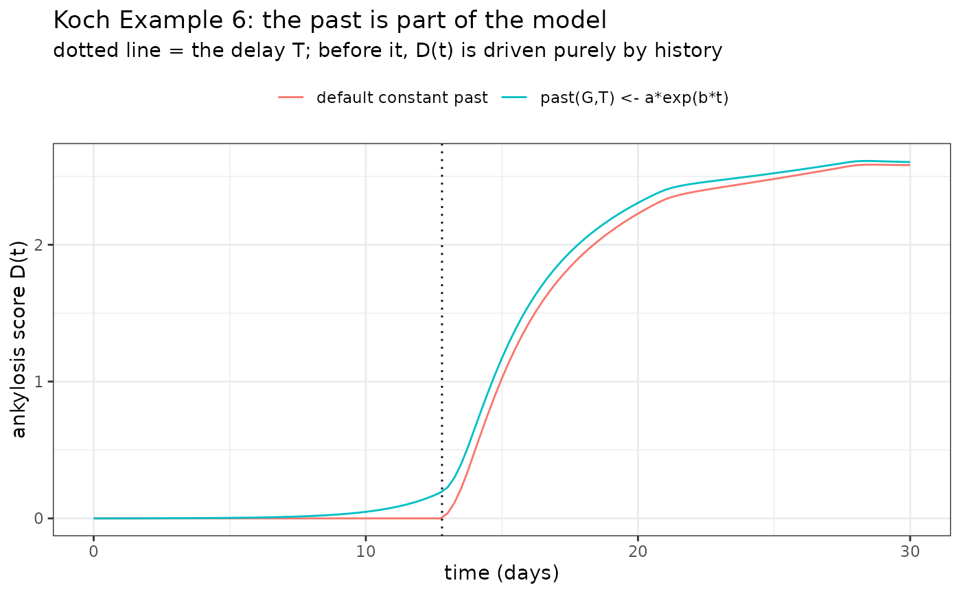

Simulating and estimating

We simulate a small population with three endpoints — PK (proportional error), TAS and AKS (additive) — dosing at days 1, 8 and 15, using the paper’s Table 5 population values.

sim6 <- rxode2({
  k  <- 0.184 * exp(eta.k)
  V  <- 0.039
  k1 <- 0.535; k2 <- 0.352; k3 <- 5
  k4 <- 0.122 * exp(eta.k4)
  k5 <- 0.126 * exp(eta.k5)
  Emax <- 1; EC50 <- 44.3
  T  <- 12.8 * exp(eta.T)
  I0 <- 2.42 * exp(eta.I0)
  a  <- 1; b <- 0.5
  d/dt(Ac) <- -k * Ac
  c   <- Ac / V
  eff <- (Emax * c) / (EC50 + c)
  G(0) <- a
  d/dt(G) <- k3 - eff * G - (k1 / k2) * (1 - exp(-k2 * t)) * G
  past(G, T) <- a * exp(b * t)
  I(0) <- I0
  d/dt(I) <- k4 * G - k4 * delay(G, T)
  D(0) <- 0
  d/dt(D) <- k4 * delay(G, T) - k5 * D
  TAS <- I + D
  AKS <- D
})

set.seed(202)
pkT <- c(1.0033, 3, 5, 7, 8.0033, 10, 15.0033, 18, 21)
pdT <- c(0, 1, 3, 5, 7, 8, 10, 12, 15, 18, 21, 25, 28)
N <- 12
ev <- et(sort(unique(c(pkT, pdT))))
for (td in c(1, 8, 15)) ev <- et(ev, amt = 1, cmt = "Ac", time = td)

rows <- list()
for (i in 1:N) {
  p <- c(eta.k = rnorm(1, 0, sqrt(0.212)), eta.k4 = rnorm(1, 0, sqrt(0.279)),
         eta.k5 = rnorm(1, 0, sqrt(0.3)),  eta.T = rnorm(1, 0, sqrt(0.0782)),
         eta.I0 = rnorm(1, 0, sqrt(0.562)))
  s <- rxSolve(sim6, params = p, ev, method = "dop853", dense = TRUE,
               returnType = "data.frame", atol = 1e-8, rtol = 1e-8)
  spk <- s[s$time %in% pkT, ]
  spd <- s[s$time %in% pdT, ]
  cdv <- spk$c * (1 + rnorm(nrow(spk), 0, 0.382)); cdv[cdv <= 0] <- 1e-3
  rows[[i]] <- rbind(
    data.frame(ID = i, TIME = spk$time, DV = cdv, AMT = 0, EVID = 0, CMT = "c"),
    data.frame(ID = i, TIME = spd$time, DV = spd$TAS + rnorm(nrow(spd), 0, 1.49),
               AMT = 0, EVID = 0, CMT = "TAS"),
    data.frame(ID = i, TIME = spd$time, DV = spd$AKS + rnorm(nrow(spd), 0, 0.420),
               AMT = 0, EVID = 0, CMT = "AKS"))
}
obs6 <- do.call(rbind, rows)
dos6 <- do.call(rbind, lapply(1:N, function(i)
  data.frame(ID = i, TIME = c(1, 8, 15), DV = NA_real_, AMT = 1, EVID = 1, CMT = "Ac")))
dat6 <- rbind(obs6, dos6)
dat6 <- dat6[order(dat6$ID, dat6$TIME, -dat6$EVID), ]

We estimate the four parameters that carry the DDE structure — the ankylosis delay T, the inflammation and destruction rates k4 and k5, and, most interestingly, b — with between-subject variability on the delay, and the three residual errors, fixing the PK and cytokine-turnover constants at the published values.

b deserves emphasis. It is the growth rate of the induction-phase history a*exp(b*t), so it appears only before $t=0$ — the model never evaluates it at any observed time point directly. It is identified purely through the history’s downstream effect on the delayed ankylosis score. Estimating it is a thing you simply cannot express without a non-constant past().

mod6 <- function() {
  ini({
    tk4 <- log(0.15)
    tk5 <- log(0.10)
    tT  <- log(11)         # delay, true 12.8
    tb  <- log(0.40)       # history growth rate, true 0.5
    eta.T ~ 0.0782
    prop.pk <- 0.382
    add.tas <- 1.49
    add.aks <- 0.420
  })
  model({
    k  <- 0.184; V <- 0.039
    k1 <- 0.535; k2 <- 0.352; k3 <- 5
    k4 <- exp(tk4)
    k5 <- exp(tk5)
    Emax <- 1; EC50 <- 44.3
    T  <- exp(tT + eta.T)
    I0 <- 2.42
    a  <- 1
    b  <- exp(tb)
    d/dt(Ac) <- -k * Ac
    c   <- Ac / V
    eff <- (Emax * c) / (EC50 + c)
    G(0) <- a
    d/dt(G) <- k3 - eff * G - (k1 / k2) * (1 - exp(-k2 * t)) * G
    past(G, T) <- a * exp(b * t)
    I(0) <- I0
    d/dt(I) <- k4 * G - k4 * delay(G, T)
    D(0) <- 0
    d/dt(D) <- k4 * delay(G, T) - k5 * D
    TAS <- I + D
    AKS <- D
    c   ~ prop(prop.pk)
    TAS ~ add(add.tas)
    AKS ~ add(add.aks)
  })
}

fit6 := nlmixr2(mod6, dat6, est = "ifoceif",
                control = foceiControl(print = 0, covMethod = "", optExpression = FALSE))
fit6

$$\begin{align*} {k} & = {0.184} \\ {V} & = {0.039} \\ {k1} & = {0.535} \\ {k2} & = {0.352} \\ {k3} & = {5} \\ {k4} & = \exp\left({tk4}\right) \\ {k5} & = \exp\left({tk5}\right) \\ {Emax} & = {1} \\ {EC50} & = {44.3} \\ {T} & = \exp\left({tT}+{eta.T}\right) \\ {I0} & = {2.42} \\ {a} & = {1} \\ {b} & = \exp\left({tb}\right) \\ \frac{d \: Ac}{dt} & = -{k} {\times} {Ac} \\ {c} & = \frac{{Ac}}{{V}} \\ {eff} & = \frac{\left({Emax} {\times} {c}\right)}{\left({EC50}+{c}\right)} \\ G({0}) & = {a} \\ \frac{dG}{dt} & = {k3}-{eff} {\times} {G}-\left(\frac{{k1}}{{k2}}\right) {\times} \left({1}-\exp\left(-{k2} {\times} {t}\right)\right) {\times} {G} \\ past({G}, {T}) & = {a} {\times} \exp\left({b} {\times} {t}\right) \\ I({0}) & = {I0} \\ \frac{dI}{dt} & = {k4} {\times} {G}-{k4} {\times} delay({G}, {T}) \\ D({0}) & = {0} \\ \frac{dD}{dt} & = {k4} {\times} delay({G}, {T})-{k5} {\times} {D} \\ {TAS} & = {I}+{D} \\ {AKS} & = {D} \\ {c} & \sim prop({prop.pk}) \\ {TAS} & \sim add({add.tas}) \\ {AKS} & \sim add({add.aks}) \end{align*}$$

truth6 <- c(k4 = 0.122, k5 = 0.126, T = 12.8, b = 0.5)
est6 <- exp(fixef(fit6)[c("tk4", "tk5", "tT", "tb")])
data.frame(parameter = names(truth6),
           truth = truth6,
           estimate = round(est6, 4),
           ratio = round(est6 / truth6, 3),
           row.names = NULL)
#>   parameter  truth estimate ratio
#> 1        k4  0.122   0.0994 0.815
#> 2        k5  0.126   0.1224 0.972
#> 3         T 12.800  13.0464 1.019
#> 4         b  0.500   0.4077 0.815

The delay T comes back close to its true 12.8 days, and — remarkably — so does the pre-history growth rate b, even though b describes cytokine dynamics that happened before the study began and are never observed directly. That a parameter of the past is estimable at all is the whole point of a non-constant past().

Practical notes

• Keep the history. A DDE interpolates its own past, so the solver has to record it. nlmixr2 arranges this for you when it sees a delay(); when you call rxSolve() yourself, pass dense=TRUE and a dense-output method such as method="dop853".
• past() is only for a non-constant history. The default pre-history is the initial condition held constant, which is what Example 2 (and most lifespan models) want. Reach for past() when the system was already running before $t=0$, as in Example 6.
• The delay is a parameter. $T$ is estimated like anything else and can carry a random effect; that is the main practical advantage over a transit chain, where the delay is implied by a rate constant and a fixed number of compartments.
• Choose the optimizer to match the delay. A delay time is a difficult parameter for a gradient-based optimizer: its exact derivative is expensive, and a finite-difference gradient is noisy because perturbing the delay slides the interpolated history. When a delay is well constrained by the data (Example 6’s ankylosis score), the gradient methods still succeed. When it is not, or when it sits inside a stiff system and a product of delayed states (Example 2), a derivative-free optimizer such as est="bobyqa" — which only evaluates the objective — is far more robust. Bounding the parameters keeps such a fit from wandering into regions where the stiff solve blows up.

Reproducing this article

The two fits here are expensive, so they are cached in inst/cache/ (shipped with the package) and reused by the website build. To refit from scratch:

cd vignettes && Rscript precompute.R --clean