Nonparametric NLME in nlmixr2 (npag/npb) versus Pmetrics (NPAG/NPOD)

nlmixr

Nonparametric population methods (`est = "npag"`, `est = "npb"`)

nlmixr2 now ships two nonparametric estimation methods:

est = "npag" – the Nonparametric Adaptive Grid (Yamada 2021), a deterministic, convex nonparametric maximum-likelihood (NPML) method; and
est = "npb" – Nonparametric Bayes, a truncated stick-breaking Dirichlet-process mixture sampled by a blocked Metropolis-within-Gibbs sampler (Tatarinova 2013; Ishwaran & James truncation).

Both estimate the entire between-subject parameter distribution as a set of discrete support points with weights, instead of assuming it is multivariate normal the way FOCEI and SAEM do. Where a parametric model summarizes between-subject variability with a single Omega matrix, a nonparametric model can represent any shape – skew, heavy tails, and, most usefully, multiple subpopulations (fast/slow metabolizers, responders/non-responders) that a single normal mode would average away.

The rest of this article leads with a worked example – the capability that makes the method worth reaching for – then, for readers who want them, the algorithm details and a step-by-step comparison with Pmetrics (the reference nonparametric package, whose pmcore engine nlmixr2’s npag is a deliberate port of) come at the end.

A note on the objective. The npag/npb objective is the nonparametric marginal log-likelihood and uses a different constant convention than NONMEM/FOCEI, so its -2LL is not comparable to nlmixr2’s FOCEI/SAEM/FOCE -2LL. Compare npag to npag, or to Pmetrics NPAG – not to a parametric objective function value.

Worked example: recovering a bimodal distribution

The defining reason to reach for a nonparametric method is a population that is not unimodal-normal. Consider an oral one-compartment drug where the absorption rate Ka comes from two subpopulations – fast and slow absorbers – with no covariate marking which is which. A parametric model with a single normal eta.ka is forced to collapse the two groups into one averaged mode with an inflated variance. NPAG is under no such constraint: it simply places support points wherever the data want mass, and the two clusters appear on their own.

Simulate two absorption subpopulations

library(nlmixr2)
set.seed(42)

nEach  <- 30L
kaSlow <- 0.7; kaFast <- 3.5          # two hidden subpopulations
vTrue  <- 30;  keTrue <- 0.1
kaTrue <- c(rep(kaSlow, nEach), rep(kaFast, nEach))

simMod <- rxode2::rxode2({
  d/dt(depot)  <- -KA * depot
  d/dt(center) <-  KA * depot - KE * center
  cp <- center / V
})
ev <- rxode2::et(amt = 100, cmt = "depot")
for (.t in c(0.25, 0.5, 1, 2, 4, 6, 8, 12, 24)) ev <- rxode2::et(ev, .t)

s   <- rxode2::rxSolve(simMod,
         data.frame(KA = kaTrue, V = vTrue, KE = keTrue), ev,
         returnType = "data.frame")
idc <- names(s)[grepl("id$", names(s), ignore.case = TRUE)][1]
obs <- s[s$time > 0, ]
obs$DV <- obs$cp + rnorm(nrow(obs), 0, 0.3)          # additive error

dat <- rbind(
  data.frame(ID = unique(obs[[idc]]), TIME = 0, DV = 0, AMT = 100, EVID = 1, CMT = 1),
  data.frame(ID = obs[[idc]], TIME = obs$time, DV = obs$DV, AMT = 0, EVID = 0, CMT = 2))
dat <- dat[order(dat$ID, dat$TIME, -dat$EVID), ]

The model

A perfectly ordinary nlmixr2 model – one random effect per structural parameter and an additive error. Nothing declares that Ka is bimodal.

oralModel <- function() {
  ini({
    tka <- log(1.5); tv <- log(30); tke <- log(0.1)
    eta.ka ~ 0.5; eta.v ~ 0.05; eta.ke ~ 0.05
    add.sd <- 0.3
  })
  model({
    ka <- exp(tka + eta.ka)
    v  <- exp(tv  + eta.v)
    ke <- exp(tke + eta.ke)
    d/dt(depot)  <- -ka * depot
    d/dt(center) <-  ka * depot - ke * center
    cp <- center / v
    cp ~ add(add.sd)
  })
}

Fit parametric (SAEM) and nonparametric (npag)

The only thing that changes between a parametric and a nonparametric fit is est =. The control settings below are deliberately small so the demonstration renders quickly (each fit is cached with :=); a production run would use the defaults.

fitSaem := nlmixr2(oralModel, dat, est = "saem",
                   control = saemControl(nBurn = 200L, nEm = 300L, print = 0L))

fitNpag := nlmixr2(oralModel, dat, est = "npag",
                   control = npagControl(points = 512L, cycles = 40L,
                                         gammaOptimize = FALSE))

SAEM returns a single eta.ka variance – the two groups are gone, folded into one wide normal mode. NPAG returns a cloud of support points (an eta vector per point, with a weight). Reconstruct Ka = exp(tka + eta.ka) from the support and look at where the weight sits:

tka       <- as.numeric(fitNpag$theta[["tka"]])
## npagSupport columns are the etas in model order; eta.ka is the first
kaSupport <- exp(tka + fitNpag$npagSupport[, 1])
weight    <- fitNpag$npagWeights

mid   <- sqrt(kaSlow * kaFast)                       # geometric-mean split
wSlow <- sum(weight[kaSupport <  mid])
wFast <- sum(weight[kaSupport >= mid])
c(slowMass = wSlow, fastMass = wFast)
#> slowMass fastMass 
#>      0.5      0.5
#> both carry substantial weight -- the two modes are recovered

## global-optimality certificate: small relative to N (= 60 subjects) means the
## support is essentially complete; a denser grid drives it further toward 0
fitNpag$env$npagDF
#> [1] 2.423211

The npag support is a set of weighted point masses; the SAEM result is a single normal mode. Overlaying them (with ggplot2) shows the contrast – the SAEM lognormal density is rescaled to the support-weight axis so both fit on one plot:

library(ggplot2)

## SAEM implied lognormal Ka density
sdKa   <- sqrt(as.numeric(fitSaem$omega["eta.ka", "eta.ka"]))
muKa   <- as.numeric(fitSaem$theta[["tka"]])
kaGrid <- seq(0.1, 6, length.out = 400)
saemDf <- data.frame(Ka = kaGrid,
                     y  = dlnorm(kaGrid, muKa, sdKa) / max(dlnorm(kaGrid, muKa, sdKa)) *
                          max(weight))
npagDf <- data.frame(Ka = kaSupport, weight = weight)

ggplot() +
  geom_vline(xintercept = c(kaSlow, kaFast), linetype = 2, colour = "grey55") +
  geom_line(data = saemDf, aes(Ka, y, colour = "SAEM (single normal mode)"),
            linewidth = 0.9) +
  geom_segment(data = npagDf,
               aes(x = Ka, xend = Ka, y = 0, yend = weight,
                   colour = "npag support (weighted points)"), linewidth = 1) +
  geom_point(data = npagDf, aes(Ka, weight, colour = "npag support (weighted points)"),
             size = 2) +
  scale_colour_manual(values = c("npag support (weighted points)" = "#2c7fb8",
                                 "SAEM (single normal mode)"       = "#d95f02"),
                      name = NULL) +
  labs(x = "Ka", y = "support weight (SAEM density rescaled)",
       title = "The two subpopulations (dashed) recovered by npag, missed by SAEM") +
  theme_bw() + theme(legend.position = "top")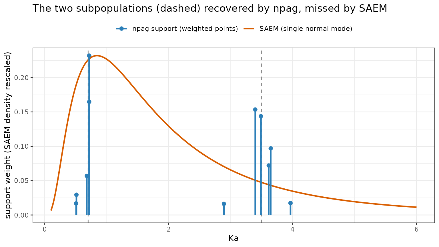

The nonparametric support shows two clean spikes near Ka = 0.7 and Ka = 3.5; the SAEM curve is one broad mode sitting in the empty valley between the subpopulations – a value no subject actually has. That gap is exactly the clinical risk a single-normal random-effect model hides.

A parametric mixture model is another way to handle exactly this situation: if you are willing to name the number of subpopulations, nlmixr2 can estimate each component’s typical parameters and the mixing probability directly – see the Mixture Models in nlmixr2 article. The difference is what you must assume. A mixture model needs the number of components chosen up front (and each component’s random effects still taken as normal), whereas the nonparametric methods discover the number and shape of the subpopulations from the data. The two are complementary: if you already know there are two absorption phenotypes and want their typical values and proportion as explicit parameters, reach for a mixture model; if you do not know how many groups there are, or suspect a more general non-normal shape, a nonparametric fit is the safer first look – and a good way to discover the structure a mixture model then names.

From support points to individual etas

So far we have the population picture: fit$npagSupport (the support points phi_k, one eta vector per row) and fit$npagWeights (their weights lambda_k), which together are the estimated mixing distribution F. How does that become each subject’s individual random effect, fit$eta?

For subject i, weight each support point by how well it explains that subject’s data – its posterior responsibility

r_ik = lambda_k * p(y_i | phi_k) / sum_j  lambda_j * p(y_i | phi_j)

– and take the responsibility-weighted average of the support points:

E[eta_i | y_i] = sum_k  r_ik * phi_k

This posterior-mean eta is stored in fit$npagPosteriorEta (one row per subject). It is the conditional expectation of the individual random effect under the actual fitted population distribution, i.e. the minimum mean-squared-error Bayes estimate. That is what makes it an appropriate individual value: because the responsibilities concentrate on the support points that match the subject, a clearly-fast absorber gets almost all its weight on the fast support points and its eta lands near the fast mode – it is not shrunk toward a global average the way a single-normal EBE would be. Reconstructing each subject’s Ka from the fit’s etas shows the two subpopulations survive at the individual level:

indKa <- exp(as.numeric(fitNpag$theta[["tka"]]) + fitNpag$eta$eta.ka)
## individual Ka splits cleanly into the two true groups
tapply(indKa, ifelse(indKa < mid, "slow", "fast"), mean)
#>      fast      slow 
#> 3.3581750 0.7463957

A note on fit$eta versus fit$npagPosteriorEta: the fit object’s eta (the ranef) are the standard empirical-Bayes estimates, recomputed by the usual MAP step under the installed normal Omega (the covariance of the support cloud) so that the nonparametric fit slots into all the ordinary tables and diagnostics. They track the nonparametric posterior means closely but are mildly shrunk toward the population mean, because that single Omega is one broad normal spanning both modes. When you want the faithful nonparametric individual value, read fit$npagPosteriorEta; for routine diagnostics fit$eta is fine.

Individual vs typical predictions – read them differently

The individual etas feed the individual predictions (IPRED), and those are excellent here: each subject’s IPRED uses its own near-mode eta, so it tracks that subject’s curve. The typical / population prediction (PRED), however, is evaluated at eta = 0 – the mean of the mixing distribution:

exp(as.numeric(fitNpag$theta[["tka"]]))      # typical Ka = the mixing-distribution mean
#> [1] 1.5

That typical Ka (about 1.5) is the valley between 0.7 and 3.5 – a “typical subject” that does not exist. So the two prediction types must be read differently. Individual predictions fit well; the typical-value prediction is a population average that is representative of no one:

d <- as.data.frame(fitNpag)
c(RMSE_PRED_vs_DV  = sqrt(mean((d$DV - d$PRED)^2)),   # typical: poor
  RMSE_IPRED_vs_DV = sqrt(mean((d$DV - d$IPRED)^2)))  # individual: good
#>  RMSE_PRED_vs_DV RMSE_IPRED_vs_DV 
#>        0.5552517        0.2856445

An augPred plot for one slow and one fast subject makes the split concrete – the Individual line hugs the observations while the Population (typical) line threads uselessly between the two subpopulations:

ap <- augPred(fitNpag)
ap <- ap[ap$id %in% c(1, 45), ]                # id 1 is slow, id 45 is fast
ggplot(ap, aes(time, values, colour = ind)) +
  geom_line(data = subset(ap, ind != "Observed"), linewidth = 0.9) +
  geom_point(data = subset(ap, ind == "Observed"), size = 1.6) +
  facet_wrap(~ id, labeller = label_both, scales = "free_y") +
  labs(x = "time", y = "concentration", colour = NULL,
       title = "Individual predictions track each subpopulation; the typical curve does not") +
  theme_bw() + theme(legend.position = "top")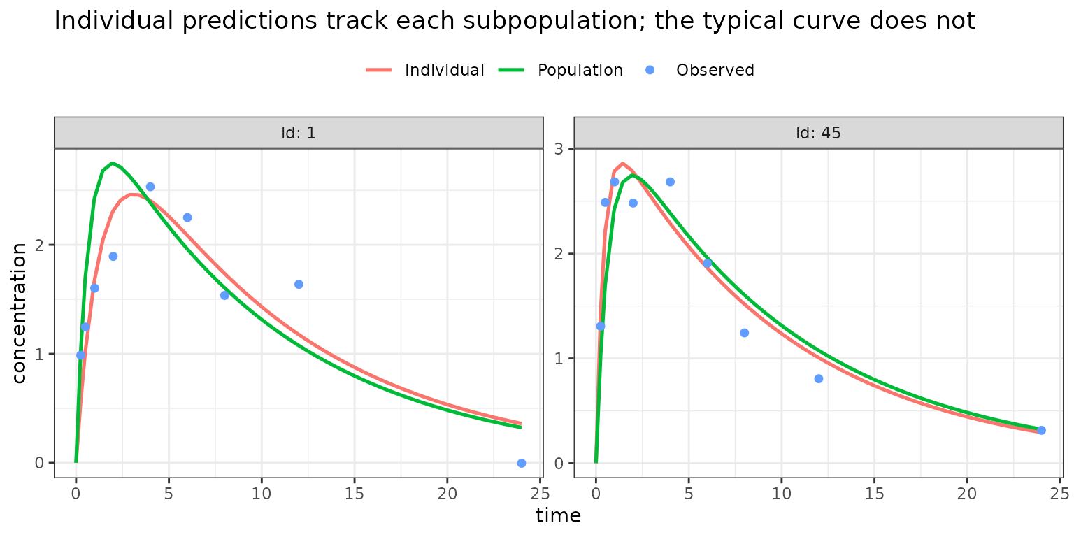

The practical guidance: for a nonparametric (potentially multimodal) fit, base goodness-of-fit on the individual diagnostics (DV vs IPRED, IWRES). PRED-based diagnostics (DV vs PRED, CWRES vs PRED) and the typical-value profile will look biased – not because the model is wrong, but because the “typical individual” is not a meaningful summary of a population made of distinct subpopulations. Treat the typical-value curve as the population-average trajectory, not as a prototype patient.

VPC and simulation – sample the support, not the normal Omega

A VPC (and any simulate() / vpcSim(), hence vpcPlot()) draws new subjects from the estimated population distribution. This is where the finalized normal Omega bites: the default nlmixr2 simulation path reads fit$simInfo$omega – the single normal covariance installed for tooling compatibility – and draws eta ~ N(0, Omega). For a multimodal population that normal is one broad unimodal spread, so it simulates virtual subjects the fit never saw.

To show it we build both simulations by hand from the same fit – the only difference is how the between-subject etas are drawn: eta ~ N(0, Omega) (the default) versus resampling whole support points by their weights (the nonparametric population the fit actually estimated, fit$npagSupport / fit$npagWeights; resampling whole rows preserves the joint eta structure):

vpcMod <- rxode2::rxode2({
  ka <- exp(tka + eta.ka); v <- exp(tv + eta.v); ke <- exp(tke + eta.ke)
  d/dt(depot)  <- -ka * depot
  d/dt(center) <-  ka * depot - ke * center
  cp <- center / v
})
obsTimes <- sort(unique(dat$TIME[dat$EVID == 0]))
evd <- rxode2::et(amt = 100, cmt = "depot"); for (tt in obsTimes) evd <- rxode2::et(evd, tt)
th <- fitNpag$theta; addSd <- as.numeric(th[["add.sd"]])

## two eta-draw rules from the SAME fit
drawNormal  <- function(n) matrix(rnorm(n * 3), n, 3) %*% chol(fitNpag$omega)   # default VPC
drawSupport <- function(n)                                                      # nonparametric
  fitNpag$npagSupport[sample(nrow(fitNpag$npagSupport), n, TRUE, fitNpag$npagWeights), , drop = FALSE]

## simulate a virtual population over the observation design
simPop <- function(drawEta, nSub, seed = 7) {
  set.seed(seed); E <- drawEta(nSub)
  pars <- data.frame(id = seq_len(nSub),
                     tka = as.numeric(th[["tka"]]), tv = as.numeric(th[["tv"]]),
                     tke = as.numeric(th[["tke"]]),
                     eta.ka = E[, 1], eta.v = E[, 2], eta.ke = E[, 3])
  sp <- rxode2::rxSolve(vpcMod, pars, evd, returnType = "data.frame")
  sp$dv <- sp$cp + rnorm(nrow(sp), 0, addSd)
  sp
}

Why the default VPC misrepresents the fit. Look at the distribution of concentrations at an early time, where Ka separates the two groups. The observed data are two clear humps; support resampling reproduces them; the default normal-Omega simulation is a single broad hump that fills the valley between them with virtual patients who do not exist:

tShow <- 0.5
popN <- simPop(drawNormal,  6000)
popS <- simPop(drawSupport, 6000)
distDf <- rbind(
  data.frame(cp = dat$DV[dat$EVID == 0 & abs(dat$TIME - tShow) < 1e-6], source = "1. observed data"),
  data.frame(cp = popS$dv[abs(popS$time - tShow) < 1e-6],               source = "2. support-based VPC"),
  data.frame(cp = popN$dv[abs(popN$time - tShow) < 1e-6],               source = "3. default VPC (normal Omega)"))
ggplot(distDf, aes(cp, fill = source)) +
  geom_histogram(aes(y = after_stat(density)), bins = 40) +
  facet_wrap(~ source, ncol = 1, scales = "free_y") +
  labs(x = paste0("concentration at t = ", tShow), y = "density",
       title = "The default VPC simulates a unimodal population the data do not have") +
  theme_bw() + theme(legend.position = "none")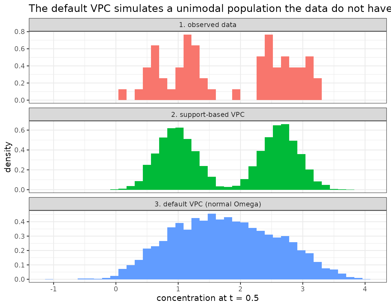


## mass in the empty valley between the two observed modes
inValley <- function(x) mean(x > 1.55 & x < 2.10)
c(observed = inValley(distDf$cp[distDf$source == "1. observed data"]),
  support  = inValley(popS$dv[abs(popS$time - tShow) < 1e-6]),
  normal   = inValley(popN$dv[abs(popN$time - tShow) < 1e-6]))
#>   observed    support     normal 
#> 0.03333333 0.02783333 0.23000000

The default VPC puts roughly a fifth of virtual subjects in the valley where the observed (and support-based) mass is near zero.

Building the actual VPC. A percentile VPC compares observed 5th/50th/95th percentiles against the simulation-based prediction intervals for those percentiles. The helper below returns those bands for either eta-draw rule:

vpcBands <- function(drawEta, nSim = 100, N = 60, seed = 3) {
  set.seed(seed); tot <- nSim * N
  E <- drawEta(tot)
  pars <- data.frame(id = seq_len(tot),
                     tka = as.numeric(th[["tka"]]), tv = as.numeric(th[["tv"]]),
                     tke = as.numeric(th[["tke"]]),
                     eta.ka = E[, 1], eta.v = E[, 2], eta.ke = E[, 3])
  sp <- rxode2::rxSolve(vpcMod, pars, evd, returnType = "data.frame")
  sp$dv <- sp$cp + rnorm(nrow(sp), 0, addSd); sp$rep <- (sp$sim.id - 1) %/% N + 1
  a  <- aggregate(dv ~ rep + time, sp, function(x) quantile(x, c(.05, .5, .95)))
  qq <- data.frame(time = a$time, lo = a$dv[, 1], med = a$dv[, 2], hi = a$dv[, 3])
  ci <- function(v) quantile(v, c(.025, .975))
  do.call(rbind, lapply(split(qq, qq$time), function(d) data.frame(time = d$time[1],
    lo_l = ci(d$lo)[1], lo_u = ci(d$lo)[2], med_l = ci(d$med)[1],
    med_u = ci(d$med)[2], hi_l = ci(d$hi)[1], hi_u = ci(d$hi)[2])))
}
band <- rbind(data.frame(vpcBands(drawNormal),  method = "default (normal Omega)"),
              data.frame(vpcBands(drawSupport), method = "support-based"))
oa  <- aggregate(DV ~ TIME, dat[dat$EVID == 0, ], function(x) quantile(x, c(.05, .5, .95)))
obsPct <- data.frame(time = oa$TIME, lo = oa$DV[, 1], med = oa$DV[, 2], hi = oa$DV[, 3])

ggplot(band, aes(time)) +
  geom_ribbon(aes(ymin = lo_l,  ymax = lo_u),  fill = "steelblue", alpha = 0.3) +
  geom_ribbon(aes(ymin = med_l, ymax = med_u), fill = "tomato",    alpha = 0.3) +
  geom_ribbon(aes(ymin = hi_l,  ymax = hi_u),  fill = "steelblue", alpha = 0.3) +
  geom_line(data = obsPct, aes(time, lo),  linetype = 2) +
  geom_line(data = obsPct, aes(time, med)) +
  geom_line(data = obsPct, aes(time, hi),  linetype = 2) +
  facet_wrap(~ method) +
  labs(x = "time", y = "concentration",
       caption = "lines = observed 5th/50th/95th; ribbons = simulated 90% CI of each") +
  theme_bw()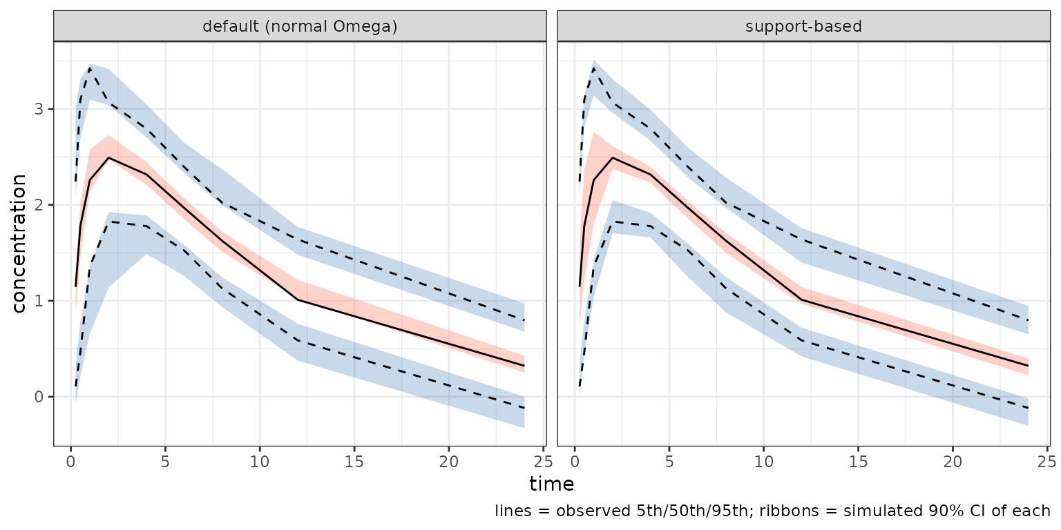

Notice the trap: at the percentile level the two VPCs look broadly similar (both roughly bracket the observed lines), so a routine percentile VPC largely hides the misrepresentation – the default panel only over-widens the peak a little. It is the distribution view above that exposes it. So:

A standard VPC of an npag/npb fit is not, on its own, a safe check for a multimodal population – it is generated from the normal Omega, not the fitted support, and its bands can look fine while the simulated population is the wrong shape.
Build the check on support resampling (fit$npagSupport / fit$npagWeights as the eta draws), as above – then the VPC is simulating from exactly the distribution the fit estimated, and is both appropriate and powerful. Inspect the simulated distribution (not only percentiles) at an informative time to confirm the shape.
When the true distribution really is unimodal, the two eta-draw rules coincide and the ordinary VPC is fine.

Add credible intervals with npb

npag tells you the two modes exist. npb tells you how sure you are, and puts credible intervals on the population summary – run several chains and check R-hat (values near 1 indicate the chains have mixed):

fitNpb := nlmixr2(oralModel, dat, est = "npb",
                  control = npbControl(points = 40L, burnin = 300L,
                                       nsamp = 300L, nchains = 3L, seed = 42L))

## posterior draws of the population-mean eta -> 95% credible intervals
apply(fitNpb$env$npbMeanDraws, 2, quantile, c(0.025, 0.5, 0.975))
#>              [,1]        [,2]        [,3]
#> 2.5%  -0.17710497 -0.04227000 -0.09596469
#> 50%    0.04110558 -0.01120577  0.04727765
#> 97.5%  0.23668901  0.05839293  0.11484211

## Gelman-Rubin R-hat per eta (~1 at convergence)
fitNpb$env$npbRhat
#>          [,1]
#> [1,] 1.001452
#> [2,] 1.353456
#> [3,] 1.582233

When to choose a nonparametric method

Reach for npag/npb when:

you suspect subpopulations (poly-morphic metabolism, responders vs non-responders, adult/pediatric mixtures) with no covariate to split them – the nonparametric distribution finds them automatically;
the between-subject distribution is plainly non-normal (skewed clearance, heavy-tailed exposure) and a normal Omega misfits the tails that drive dosing;
you are doing MAP-Bayesian / model-informed precision dosing and want an empirical prior that matches the real (possibly multimodal) population rather than a smooth normal one – the Pmetrics lineage of these methods was built precisely for individualized dosing;
you want a global-optimum guarantee on the mixing distribution (the convex weight problem plus the npagDF certificate) rather than a local optimum;
(with npb) you need posterior uncertainty on the population distribution itself, not just a point estimate.

Stick with FOCEI/SAEM when the normal-random-effect assumption is reasonable and you want the smallest, most familiar parameterization, an objective function comparable across parametric runs, and the fastest fit. The nonparametric methods trade some of that speed and comparability for the ability to see a population shape the parametric model cannot represent.

For a known number of subpopulations there is a middle path: a parametric mixture model, which names each component’s typical parameters and the mixing proportion explicitly (still assuming normal within-component random effects). Use a mixture model when the number of groups is known and you want them as explicit parameters; use npag/npb when the number and shape of the groups are themselves in question – or use a nonparametric fit first to reveal the structure and a mixture model to formalize it.

The remainder of this article is the algorithm reference: how the adaptive grid works, how npb differs, and how the nlmixr2 implementation compares with Pmetrics step by step. Skip it unless you want the internals.

How the adaptive grid works

The nonparametric maximum-likelihood problem

Let p(y_i | theta) be the likelihood of subject i’s data at a single parameter vector theta (obtained by solving the model ODE for that subject and evaluating the residual-error model). A nonparametric population model represents the population as a discrete mixing distribution

F = sum_k  w_k * delta(theta_k),      w_k >= 0,   sum_k w_k = 1

– a cloud of support points theta_k carrying probability weights w_k. The marginal likelihood of the whole population is

L(F) = prod_i  ( sum_k  w_k * p(y_i | theta_k) )

The remarkable theoretical result (Lindsay 1983; Mallet 1986) is that the NPML estimate F-hat is discrete with at most N support points (N = number of subjects), and, for a fixed set of candidate points, maximizing L(F) over the weights w is a convex problem with a unique solution. NPAG alternates between:

solving the convex weight problem on the current grid (an interior-point solve), and
moving/adding grid points toward regions the data want more density (the adaptive part),

until the likelihood stops improving. Because step 1 is convex, the method has no local-minimum problem in the weights; the only search is over where to put the support points.

The NPAG cycle

One NPAG cycle, as implemented in both pmcore and nlmixr2, is the loop below (rendered with DiagrammeR). The diamonds are the convergence controller: the cycle repeats at the current grid resolution until the objective stalls, then halves eps and repeats, and only stops when halving no longer helps.

Estimation – build the Psi matrix Psi[i, k] = p(y_i | theta_k) (subjects x support points), then solve for the maximum-likelihood weights with Burke’s primal-dual interior-point method.
Condensation – discard support points that carry negligible weight (w_k <= max(w)/1000), then run a rank-revealing QR on the row-normalized Psi to drop points that are numerically redundant (linearly dependent columns). This keeps the grid from exploding.
Error-model optimization – nudge the residual-error magnitude up and down and keep whichever improves the likelihood.
Evaluation – when the objective stops changing at the current grid resolution, halve the grid step eps (from an initial 0.2 down to a floor of 1e-4). When halving no longer helps either, the fit has converged.
Expansion – at the start of the next cycle, place up to two daughter points per dimension around every surviving support point, at +/- eps * range, discarding any that fall outside the box or land too close to an existing point.

Both packages share the exact tuning constants: eps starts at 0.2; the objective-change tolerance that triggers eps-halving is 1e-4; the eps floor is 1e-4; the successive-likelihood exit tolerance is 1e-2; the minimum scaled daughter-point distance is 1e-4.

Global optimality: the D(F) certificate

Because the weight problem is convex, there is a certificate for having found the global NPML optimum (Yamada 2021, Sec. 2.9). Define the directional derivative

D(theta, F) = sum_i  p(y_i | theta) / p(y_i | F)  -  N

At the true optimum, max_theta D(theta, F) ~ 0; a large positive value means the grid missed a mode and is not the global optimum. nlmixr2 reports this as fit$env$npagDF (computed over a fresh Sobol scan of the box), the value printed in the example above. It is a one-time diagnostic that does not change the fit – a near-zero value is your evidence that the support is complete.

The likelihood: reusing the FOCEI inner evaluation

nlmixr2’s npag/npb do not carry their own likelihood code. They fill each Psi[i, k] = p(y_i | phi_k) by reusing the FOCEI inner evaluation (src/inner.cpp): the model is solved at the support point’s etas phi_k and the per-observation log-likelihoods are summed. Two consequences follow – one reassuring, one to keep in mind – and together they set out when the method is appropriate.

What it does not import: the FOCEI marginal approximation. FOCEI’s well-known approximation error comes from the Laplace linearization it uses to integrate over the random effects when forming the marginal likelihood. NPAG/NPB never do that integral by linearization – they marginalize by the discrete sum sum_k lambda_k p(y_i | phi_k), which is exact for a discrete mixing distribution, and each p(y_i | phi_k) is evaluated at a fixed eta (the support point), so it is the exact conditional density (the inner routine even drops the Omega prior term, since the nonparametric weights lambda_k replace it). Reusing the FOCEI inner routine therefore borrows only the exact per-point likelihood, not the approximate marginalization. This is a genuine advantage over FOCEI for sparse or strongly nonlinear data, where the Laplace approximation to the marginal is poor: the nonparametric marginal likelihood is exact given the support.

What it does import: rxode2’s residual model, and its convention. Because the per-point density is the rxode2/FOCEI inner one, npag/npb inherit – for free – every rxode2 residual-error model (additive/proportional/combined, lnorm, transform-both-sides, autocorrelation), M2/M3/M4 censoring, and even user ll() general likelihoods (there the summed llikObs is exactly the user’s log-likelihood, so the nonparametric objective is immediately correct for non-normal data). The flip side is threefold: (1) the likelihood is only as faithful as that inner residual evaluation; (2) it carries the FOCEI conditional-density constant convention, so the reported -2LL is not comparable to a parametric FOCEI/SAEM run or to Pmetrics’ constant – compare npag to npag; and (3) the residual-error parameters themselves are estimated by an approximate extended-least-squares step at the posterior-mean etas (not by the exact marginal), a deliberate trade for speed and stability on a flexible support.

Appropriateness. The construction is sound whenever the conditional likelihood is trustworthy at a fixed parameter vector – exactly the regime PK/PD models are built for. It is the right tool when you want an exact treatment of a non-normal or multimodal between-subject distribution without paying FOCEI’s marginal-approximation error. It is not a route to a smaller or NONMEM-comparable objective function; and, as the simulation/VPC and typical-prediction sections showed, the normal-Omega summary the fit finalizes into must not be mistaken for the population it came from.

Relationship to `impmap`

npagControl() and npbControl() are thin wrappers around impmapControl(): each builds an impmap control, tags it with its own est, and layers the nonparametric fields (points, cycles, gridWidth, alpha, …) on top. Anything you pass through ... goes to impmapControl(). That is a deliberate reuse, and it is worth knowing exactly how far it goes.

What npag/npb genuinely share with impmap. The whole FOCEI-family scaffolding: the inner MAP problem that produces each subject’s conditional mode, mu-referencing, the Omega/eta plumbing, the residual-error machinery, mixture proportions, iteration printing, and the thread count. In the C++ layer the nonparametric kernels call the same imp* interface (impMapPass, impSetEta, impGetOmega, impMuInterceptStep, impIterPrint*) that the importance-sampling EM does.

What they do not share: the E-step. impmap draws importance samples from a parametric proposal centred at each subject’s MAP mode and updates by EM. npag/npb replace that entirely – with an adaptive grid over support points, or with a Dirichlet-process posterior. Neither calls impEStep.

That distinction has a practical consequence, and the package now tells you about it rather than leaving you to find out.

When a control does not apply, you get told

The importance-sampling controls configure a proposal density that a nonparametric engine never builds. Passing one used to be accepted and silently ignored – so a fit could be “tuned” with knobs that did nothing. It is now an error, and the error names the control that does do the job:

npagControl(nIter = 200)
#> Error: use 'cycles' instead of 'nIter'

npagControl(isample = 500)
#> Error: 'isample' configure the importance-sampling proposal,
#>        which est="npag" does not build

npbControl(impSeed = 7)
#> Error: use 'seed' instead of 'impSeed'

So there is nothing to memorise. If you reach for an impmap habit, you find out immediately. The handful with a direct counterpart:

you reach for	`npag`/`npb` control	why
`nIter`	`cycles`	npag counts adaptive-grid cycles, not EM iterations
`ctol`, `nConvWindow`	`rhoend`, `cycles`	convergence is the grid’s, not an EM window’s
`impSeed`	`seed` (npb)	npag needs none – its grid is Sobol-deterministic
`gamma`	`gammaOptimize`	unrelated quantities that happen to share a word – see below

Everything else in that family (isample, df, auto, iaccept, iscaleMin, iscaleMax, qr, sir and the rest) has no nonparametric counterpart at all, because there is no proposal to shape. The controls that do steer npag are points, cycles, gridWidth, gridBounds and residOptimize; for npb, points, alpha, burnin, nsamp, nchains, propSd and seed.

The shared FOCEI-family scaffolding still passes through untouched – the residual error model, covMethod, sigdig, the thread count and so on – since that half of the inheritance is real.

A word that means two things

gamma and gammaOptimize are unrelated:

control	method	meaning
`gamma`	`impmap`	proposal-variance inflation (NONMEM `ISCALE`); scales the proposal covariance
`gammaOptimize`	`npag`/`npb`	a global assay-error multiplier on the residual magnitude, in the Pmetrics sense

This one is worth a sentence of its own because R would otherwise do something surprising with it. gamma is a prefix of gammaOptimize, so R’s partial argument matching once bound npagControl(gamma = 2) to gammaOptimize, setting it to isTRUE(2) – that is, FALSE. Reaching for impmap’s proposal control did not get ignored; it silently switched the assay-error optimisation off. gamma is now rejected by name, so the partial match cannot happen.

Choosing between them. Both handle a between-subject distribution that a normal Omega cannot; they answer different questions. impmap keeps a parametric Omega and improves how the marginal likelihood is integrated (exactly the FOCEI approximation error). npag/npb drop the normal assumption on the distribution itself and estimate it as a discrete measure. If your structural model is fine and you distrust the Laplace marginal, reach for impmap; if you suspect the population is multimodal or otherwise not normal in eta space, reach for npag. The diagnostic that tells you impmap is struggling – Pareto k-hat, fit$env$impPsisK – has no counterpart here, because there is no importance-sampling proposal whose tails could fail.

The npb (Nonparametric Bayes) method

npag gives a point estimate of the mixing distribution. npb instead puts a Dirichlet-process prior on it and samples the posterior, so you get credible intervals on the population mean and on every support point – something npag can only get through bootstrap.

The nonparametric Bayes method (npb) is not a separate lineage bolted on after the fact: it was introduced in the same paper as NPAG – Tatarinova et al. (2013), Two general methods for population pharmacokinetic modeling: nonparametric adaptive grid and nonparametric Bayesian – which presented the adaptive grid and this Bayesian mixture side by side as two complementary answers to the same nonparametric estimation problem. nlmixr2 follows that pairing: npag and npb share the conditional-likelihood primitive and the fit finalization, and differ only in how the support points and weights are drawn.

The model is a truncated stick-breaking mixture: phi_k ~ G0, v_k ~ Beta(1, alpha), w_1 = v_1, w_k = v_k * prod_{j<k}(1 - v_j), truncated at K points, with base measure G0 = N(0, diag(Omega_prior)) in eta space. Each blocked Gibbs sweep does:

cluster assignment – z_i ~ Categorical(w_k * p(y_i | phi_k));
stick weights – v_k | counts ~ Beta(1 + n_k, alpha + sum_{j>k} n_j);
support locations – a Gaussian random-walk Metropolis step on each occupied cluster’s phi_k against G0 and its assigned subjects’ likelihoods.

Post-burn-in draws give the posterior mixing distribution, per-subject posterior-mean etas, posterior draws of the population mean (for credible intervals), and, with nchains > 1, a Gelman-Rubin R-hat per parameter.

npb is not a Pmetrics method. Pmetrics’ third algorithm, POSTPROB, is a single reweighting of a fixed prior distribution to new data/error model (useful for MAP-Bayesian dosing against an existing nonparametric prior), which is a different tool than a full Bayesian mixture posterior.

Interpreting an npb fit – the same caveats, plus posterior uncertainty

npb shares the conditional-likelihood primitive and the fit finalization with npag, so every interpretation point from the worked example carries over, through the parallel accessors fit$npbSupport, fit$npbWeights, and fit$npbPosteriorEta:

Support to eta. A subject’s fit$eta is again the empirical-Bayes estimate under the installed normal Omega (here the posterior-mean support covariance), so it is mildly shrunk relative to the faithful nonparametric posterior mean in fit$npbPosteriorEta.
Individual vs typical predictions. IPRED uses the near-mode individual eta and tracks each subpopulation; PRED sits at the – possibly unrepresentative – mixing-distribution mean. Lean on IPRED-based diagnostics.
VPC and simulation. The default simulate() / vpcSim() / vpc() path draws from the normal Omega, so a faithful VPC must resample the posterior support (fit$npbSupport / fit$npbWeights) instead – exactly as for npag.

npb adds one capability npag lacks here: because it retains posterior draws of the whole mixing distribution (fit$npbMeanDraws, and the pooled posterior support), a simulation can propagate the posterior uncertainty in the population distribution – not just resample a single point estimate of it – so a posterior-predictive check can carry both the between-subject spread and the uncertainty about that spread.

How nlmixr2 compares with Pmetrics, step by step

The following table maps each step of the adaptive-grid cycle across the two implementations. “Same” means the algorithm and constants are identical (the nlmixr2 port follows pmcore deliberately); “Differs” flags a genuine design choice.

Step	Pmetrics / `pmcore` 0.25.2 (Rust)	`nlmixr2est` `est="npag"` (C++)	Same / Differs
Parameter space	Points are native structural parameters (Ke, V, …). Every parameter is nonparametric; there is no fixed/random split.	Points are eta (random-effect) deviations; the structural value is `theta + eta`. Only mu-referenced params get a distribution; a non-mu structural param is a point estimate (a “regressor”).	Differs (fundamental)
Support box	User must supply finite `[lower, upper]` on every parameter; infinite bounds error out.	Box is derived automatically: `+/- gridWidth * eta SD` (`gridWidth=4`), or the `ini` block bounds (`gridBounds="ini"/"both"`). No user ranges required.	Differs
Initial grid	Sobol sequence (`sobol_burley`), default 2028 points, seed 22, scaled to the parameter box.	Sobol sequence (`boost::random::sobol`), default `max(2028, 512 * n_eta)`, scaled to the eta box.	Differs (auto grows with dimension)
Likelihood `Psi[i,k]`	`pharmsol` solves the ODE per subject x point and evaluates a polynomial assay-error likelihood (`log_likelihood_matrix`).	Reuses the FOCEI inner engine (`src/inner.cpp`): sums the per-observation `llikObs`, inheriting rxode2 error models, transform-both-sides and M2/M3/M4 censoring unchanged.	Differs (engine), same quantity
Weight solver	Burke primal-dual IPM (`ipm.rs`), `faer` Cholesky, no iteration cap.	Burke IPM ported line-for-line (`npCommon.cpp`), Armadillo Cholesky, plus a ridge-retry on non-PD Newton matrices, an iteration cap, and per-row log-sum-exp normalization to avoid underflow.	Same algorithm, hardened
Condensation 1 (weight)	Keep `w_k > max(w)/1000`.	Keep `w_k > max(w)/1000` (`ratio = 1e-3`).	Same
Condensation 2 (QR)	Column-pivoted rank-revealing QR on row-normalized `Psi`; keep column `i` if `\|R_ii\| / \|\|R col i\|\| >= 1e-8`.	Same, via Eigen `ColPivHouseholderQR`, `tol = 1e-8`.	Same
Error-model optimization	Scale one gamma/lambda multiplier per output equation up/down by `(1 +/- delta)`; keep the better; `delta = 4` on success, `= 0.5` otherwise. The assay-error polynomial `C0..C3` is user-fixed.	Same gamma up/down warm start, then a full residual-theta optimization: every `add`/`prop`/`lnorm`/`lambda`/`ar` is fit by bounded `bobyqa` on an extended-least-squares objective at the posterior-mean etas (the `log(r)` term stops the residual collapsing on a flexible support). gamma is folded into the coefficients at the end.	Differs (nlmixr2 does much more)
Expansion	Adaptive grid: `+/- eps * range` per dimension; discard daughters within `min_dist` (normalized L2) of an existing point or outside the box.	Same, `npExpandGrid`; `min_dist` uses a normalized L1 distance.	Same (minor metric diff)
Convergence controller	eps `0.2 -> 1e-4` by halving; converge when successive offset-cycle log-likelihoods differ by `< 1e-2`.	Identical constants and logic.	Same
Global-optimality certificate	Used internally (NPOD steers expansion by the D-gradient); not surfaced as a single number by NPAG.	`D(F)` scan reported as `npagDF` (Yamada Sec. 2.9).	Differs (reported)
Finalization	Returns the fully nonparametric result (`support`, `weights`, cycle log); stays nonparametric end to end.	Summarizes the discrete distribution into a population mean (mu-referenced `theta` shift) `+ Omega`, pushes them into FOCEI state, computes posterior-mean etas, and builds a standard `nlmixr2FitData` – a nonparametric fit that plugs into the parametric tooling (tables, `$parFixed`, covariance, diagnostics). The discrete support is kept alongside.	Differs (hybrid output)
Runtime	Standalone Rust; model compiled to a shared library; own ODE solver (`diffsol`) + rayon threads.	In-process C++/RcppArmadillo; model compiled to rxode2 C; rxode2/OpenMP threads.	Differs (host)

The “second” nonparametric method differs by design

The two packages take different second methods, so this pairing is not a port:

Aspect	Pmetrics NPOD	`nlmixr2` `npb`
Family	Nonparametric Optimal Design (Leary/Bustad): grid-free NPML.	Nonparametric Bayes: Dirichlet-process mixture.
Estimation	Same convex Burke weight solve; expansion replaces the fixed `+/- eps` grid with a local optimizer (`SppOptimizer`) that moves each candidate to the maximizer of the D-gradient `D(theta, F)`.	Blocked Metropolis-within-Gibbs sampler over cluster assignments, stick weights, and support locations.
Output	A point NPML estimate reached with far fewer support-point evaluations than a dense grid.	A full posterior: credible intervals on the mean and support, R-hat convergence.
Convergence	D-function optimality, like NPAG.	MCMC diagnostics (Gelman-Rubin).
Counterpart	No `nlmixr2` equivalent yet.	No Pmetrics equivalent (POSTPROB only reweights a fixed prior).

So the honest mapping is: NPAG is shared (a deliberate port), while Pmetrics’ NPOD and nlmixr2’s npb are different answers to “what else can we do nonparametrically” – NPOD makes the grid smarter, npb makes the estimate Bayesian.

Why the parameter-space choice matters most

The single most consequential difference is native-parameter space (Pmetrics) versus eta space (nlmixr2):

Pmetrics has no fixed effects. Every parameter carries a full distribution, so the population “mean” is just a summary of the support cloud. You must give each parameter a physiologically sensible finite range.
nlmixr2 layers the nonparametric grid on top of its mu-referencing machinery. A mu-referenced parameter keeps a typical value (theta) and only its deviation (eta) is nonparametric; the grid box comes from the initial eta variance. A structural parameter with no eta stays a point estimate, optimized as a “regressor”. This is why an nlmixr2 nonparametric fit drops straight into the same fit object, tables, and plots as a FOCEI/SAEM fit – and why its -2LL constant convention differs from a parametric run.

Practically: a pure Pmetrics workflow expresses everything as a distribution; the nlmixr2 workflow lets you make some parameters nonparametric (the ones with etas) while others stay classical, inside one model syntax.

References

Yamada WM, et al. An Algorithm for Nonparametric Estimation of a Multivariate Mixing Distribution With Applications to Population Pharmacokinetics. Pharmaceutics, 2021.
Burke JV, Ye Y. A primal-dual interior-point method for the nonparametric maximum-likelihood problem (as implemented in pmcore ipm.rs).
Lindsay BG. The geometry of mixture likelihoods. Ann. Statist., 1983; Mallet A. A maximum likelihood estimation method for random coefficient regression models. Biometrika, 1986.
Tatarinova T, et al. Two general methods for population pharmacokinetic modeling: nonparametric adaptive grid and nonparametric Bayesian. J. Pharmacokinet. Pharmacodyn., 2013.
Neely MN, et al. Accurate Detection of Outliers and Subpopulations With Pmetrics. Ther. Drug Monit., 2012. Pmetrics; pmcore crate: https://crates.io/crates/pmcore. ```

2026-09-15

Nonparametric population methods (est = "npag", est = "npb")