nlmixr
Adding Covariances between random effects
You can simply add co-variances between two random effects by adding
the effects together in the model specification block, that is
eta.cl+eta.v ~. After that statement, you specify the lower
triangular matrix of the fit with c().
An example of this is the phenobarbitol data:
Model Specification
pheno <- function() {
  ini({
    tcl <- log(0.008) # typical value of clearance
    tv <-  log(0.6)   # typical value of volume
    ## var(eta.cl)
    eta.cl + eta.v ~ c(1,
                       0.01, 1) ## cov(eta.cl, eta.v), var(eta.v)
                      # interindividual variability on clearance and volume
    add.err <- 0.1    # residual variability
  })
  model({
    cl <- exp(tcl + eta.cl) # individual value of clearance
    v <- exp(tv + eta.v)    # individual value of volume
    ke <- cl / v            # elimination rate constant
    d/dt(A1) = - ke * A1    # model differential equation
    cp = A1 / v             # concentration in plasma
    cp ~ add(add.err)       # define error model
  })
}
Fit with SAEM
fit <- nlmixr(pheno, pheno_sd, "saem",
control=list(print=0),
table=list(cwres=TRUE, npde=TRUE))
#> [====|====|====|====|====|====|====|====|====|====] 0:00:00
#> [====|====|====|====|====|====|====|====|====|====] 0:00:00
#> [====|====|====|====|====|====|====|====|====|====] 0:00:00
#> [====|====|====|====|====|====|====|====|====|====] 0:00:00
#> [====|====|====|====|====|====|====|====|====|====] 0:00:00
#> [====|====|====|====|====|====|====|====|====|====] 0:00:00
#> [====|====|====|====|====|====|====|====|====|====] 0:00:00
#> [====|====|====|====|====|====|====|====|====|====] 0:00:00
#> [====|====|====|====|====|====|====|====|====|====] 0:00:00
#> [====|====|====|====|====|====|====|====|====|====] 0:00:00
#> [====|====|====|====|====|====|====|====|====|====] 0:00:00
#>
#> [====|====|====|====|====|====|====|====|====|====] 0:00:00
#>
#> [====|====|====|====|====|====|====|====|====|====] 0:00:00
#> [====|====|====|====|====|====|====|====|====|====] 0:00:00
#> [====|====|====|====|====|====|====|====|====|====] 0:00:00
#> [====|====|====|====|====|====|====|====|====|====] 0:00:00
#> [====|====|====|====|====|====|====|====|====|====] 0:00:00
#> [====|====|====|====|====|====|====|====|====|====] 0:00:00
#> [====|====|====|====|====|====|====|====|====|====] 0:00:00
#> [====|====|====|====|====|====|====|====|====|====] 0:00:00
#> [====|====|====|====|====|====|====|====|====|====] 0:00:00
#> [====|====|====|====|====|====|====|====|====|====] 0:00:00
#> [====|====|====|====|====|====|====|====|====|====] 0:00:00
#> [====|====|====|====|====|====|====|====|====|====] 0:00:00
#>
#> [====|====|====|====|====|====|====|====|====|====] 0:00:00
#>
#> [====|====|====|====|====|====|====|====|====|====] 0:00:00
#> [====|====|====|====|====|====|====|====|====|====] 0:00:00
#> [====|====|====|====|====|====|====|====|====|====] 0:00:00
#> [====|====|====|====|====|====|====|====|====|====] 0:00:00
#> [====|====|====|====|====|====|====|====|====|====] 0:00:00
print(fit)
#> ── nlmixr² SAEM OBJF by FOCEi approximation ──
#>
#> OBJF AIC BIC Log-likelihood Condition#(Cov) Condition#(Cor)
#> FOCEi 689.3203 986.1912 1004.452 -487.0956 6.033342 5.252589
#>
#> ── Time (sec $time): ──
#>
#> setup optimize covariance saem table compress
#> elapsed 0.004834 1.6e-05 0.020017 9.284 2.358 0.084
#>
#> ── Population Parameters ($parFixed or $parFixedDf): ──
#>
#> Est. SE %RSE Back-transformed(95%CI) BSV(CV%) Shrink(SD)%
#> tcl -5.02 0.075 1.5 0.00663 (0.00573, 0.00769) 51.8 3.26%
#> tv 0.35 0.0548 15.7 1.42 (1.27, 1.58) 41.9 1.40%
#> add.err 2.76 2.76
#>
#> Covariance Type ($covMethod): linFim
#> Correlations in between subject variability (BSV) matrix:
#> cor:eta.v,eta.cl
#> 0.946
#>
#>
#> Full BSV covariance ($omega) or correlation ($omegaR; diagonals=SDs)
#> Distribution stats (mean/skewness/kurtosis/p-value) available in $shrink
#> Censoring ($censInformation): No censoring
#>
#> ── Fit Data (object is a modified tibble): ──
#> # A tibble: 155 × 26
#> ID TIME DV EPRED ERES NPDE NPD PDE PD PRED RES WRES
#> <fct> <dbl> <dbl> <dbl> <dbl> <dbl> <dbl> <dbl> <dbl> <dbl> <dbl> <dbl>
#> 1 1 2 17.3 18.9 -1.58 -0.350 -0.0920 0.363 0.463 17.5 -0.162 -0.0214
#> 2 1 112. 31 29.7 1.25 0.245 0.245 0.597 0.597 28.0 2.98 0.244
#> 3 2 2 9.7 11.4 -1.71 -0.664 -0.202 0.253 0.42 10.5 -0.777 -0.154
#> # ℹ 152 more rows
#> # ℹ 14 more variables: IPRED <dbl>, IRES <dbl>, IWRES <dbl>, CPRED <dbl>,
#> # CRES <dbl>, CWRES <dbl>, eta.cl <dbl>, eta.v <dbl>, A1 <dbl>, cl <dbl>,
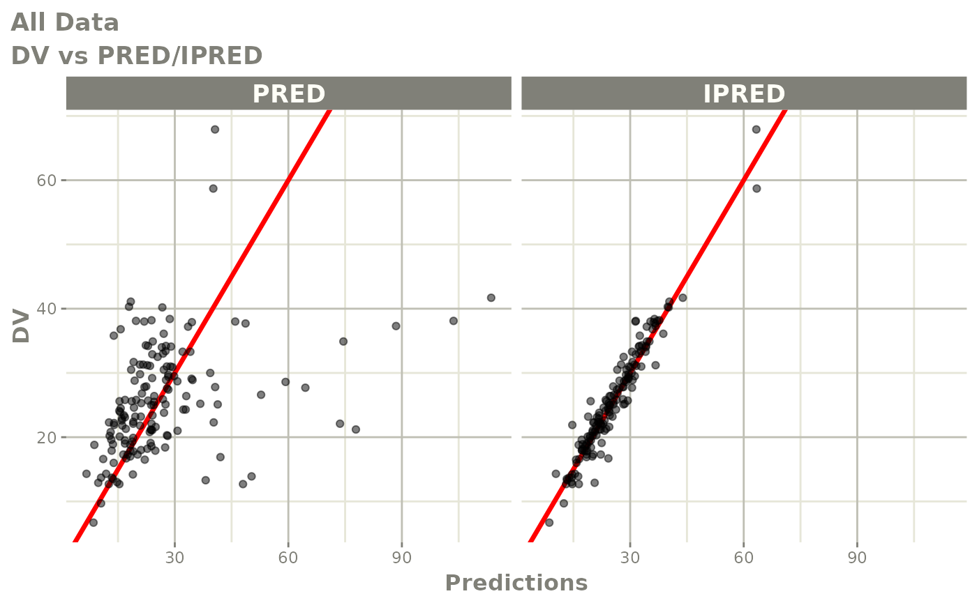
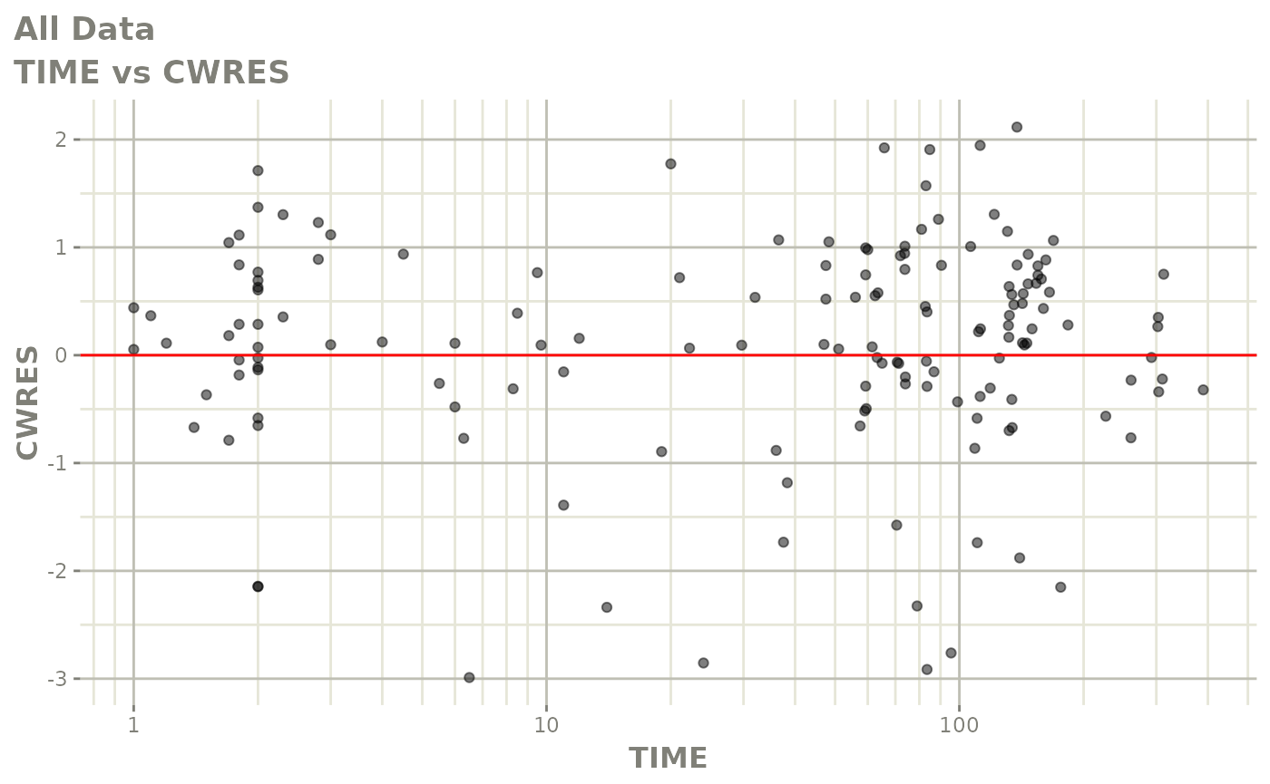
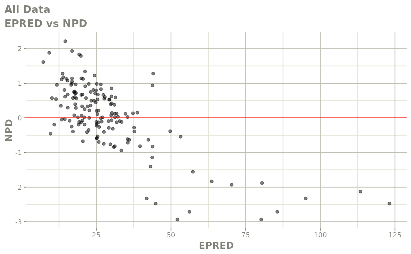
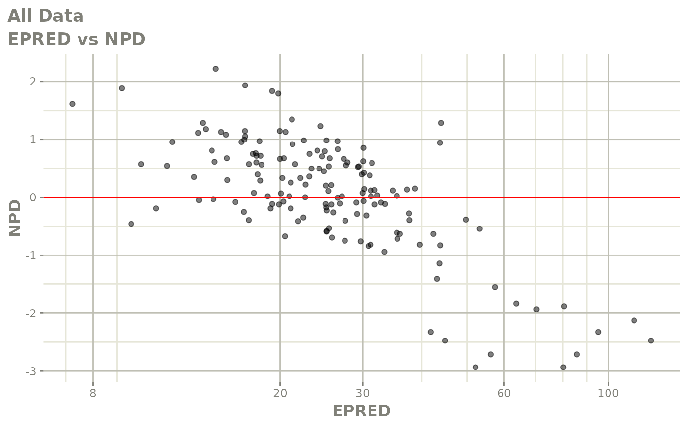
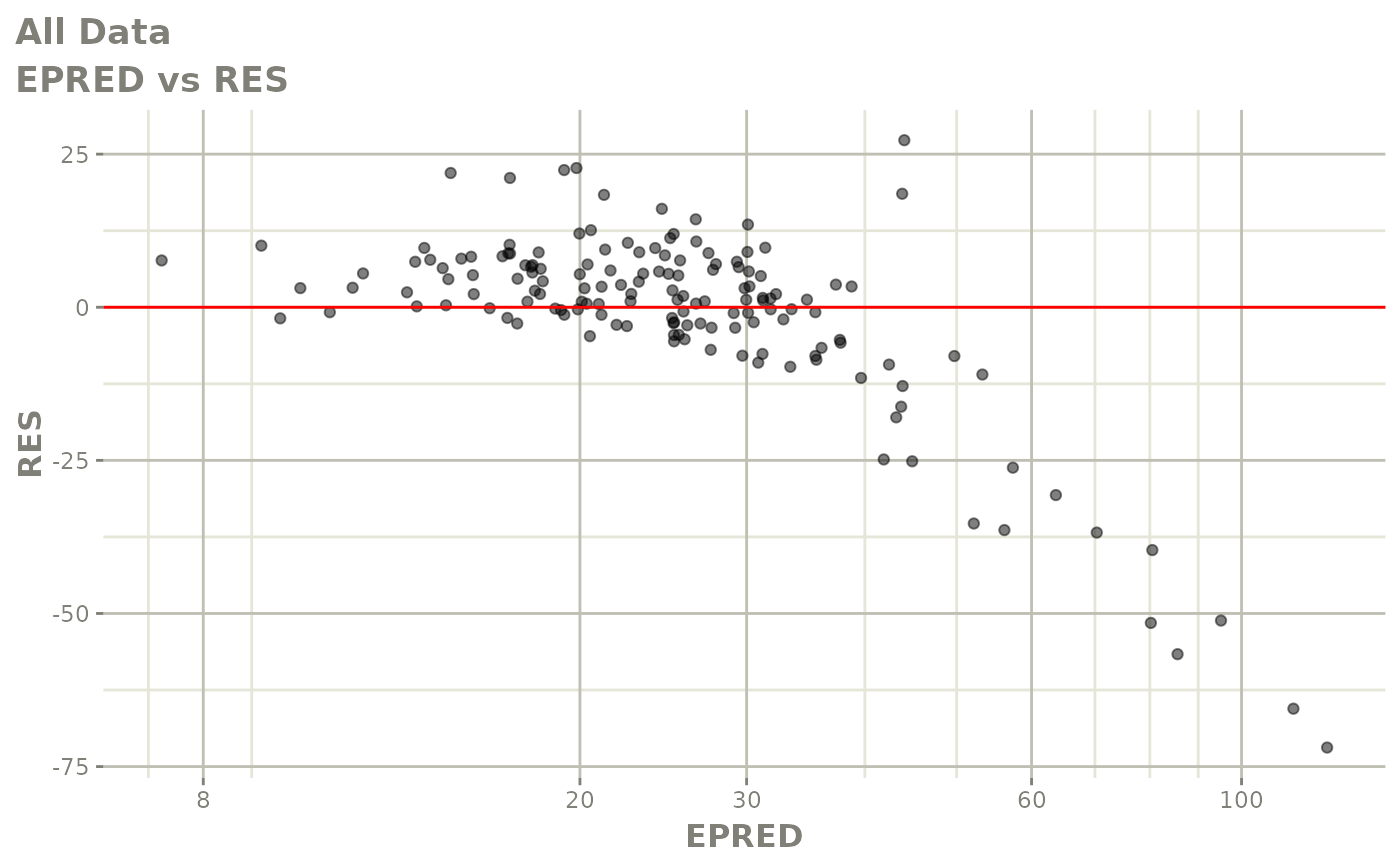
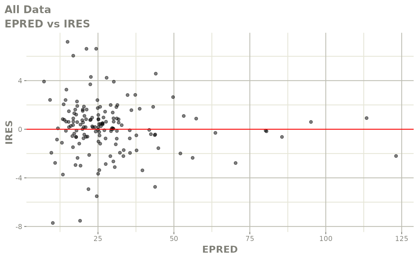
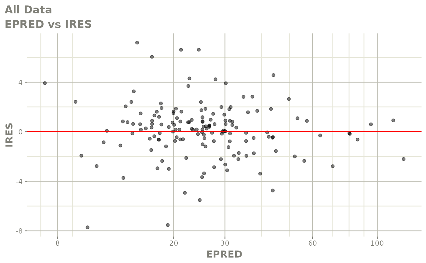
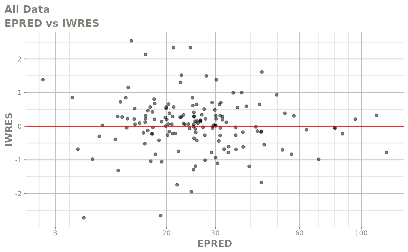
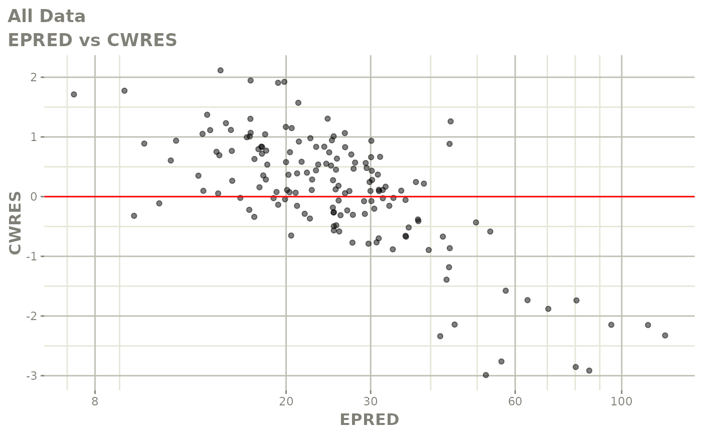
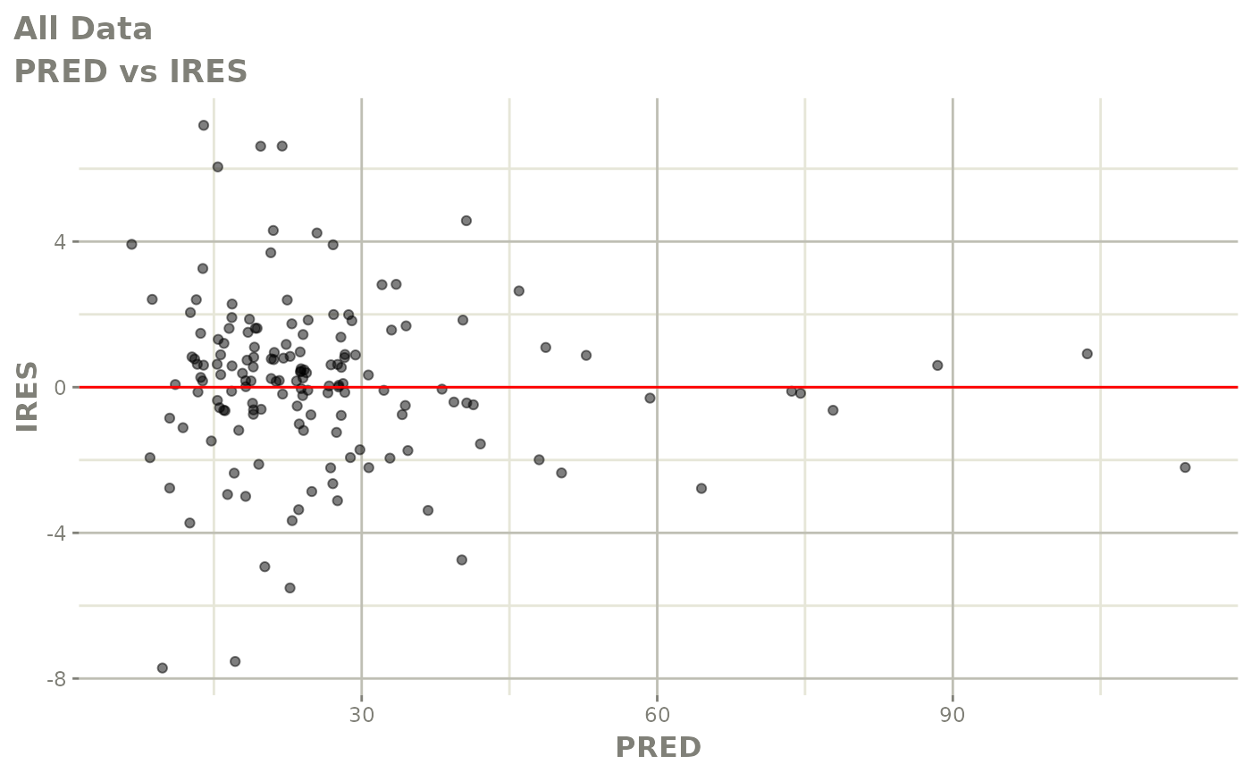
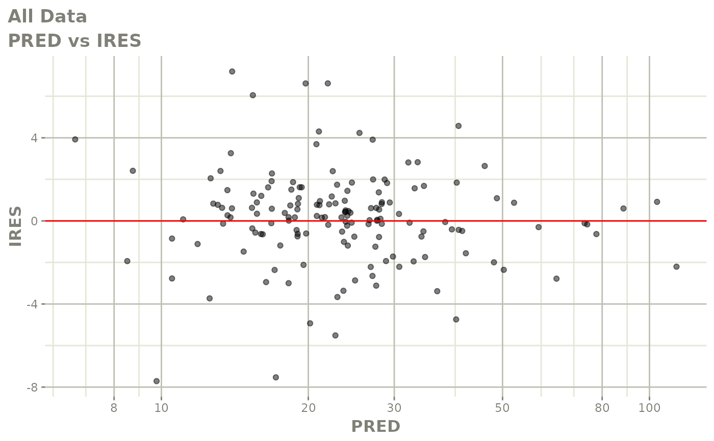
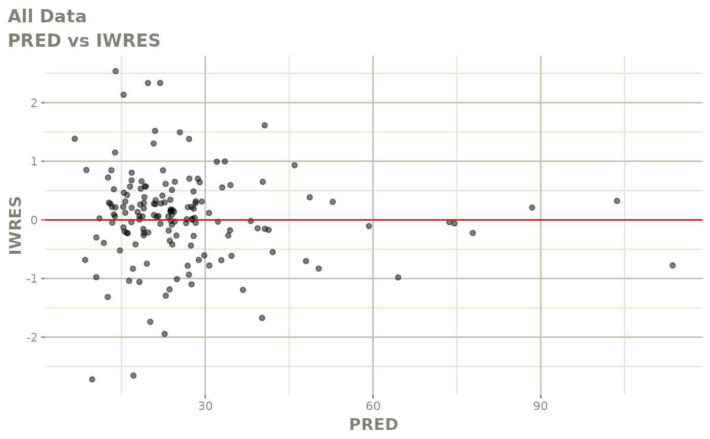
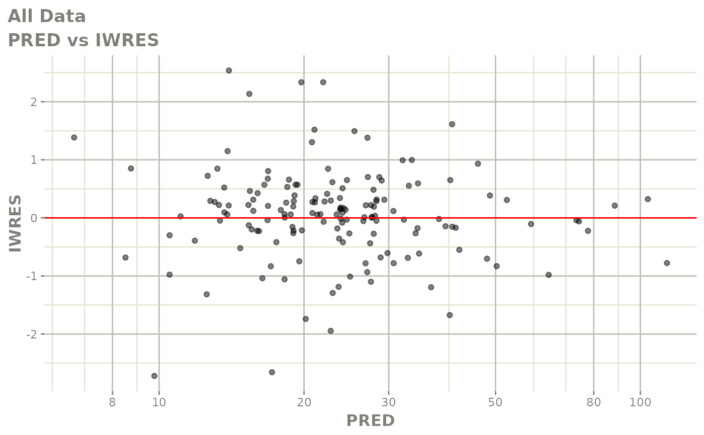
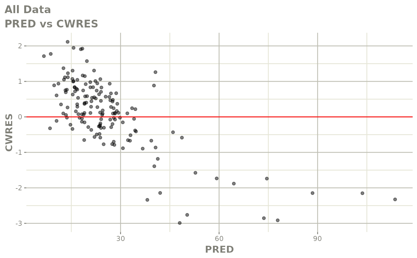
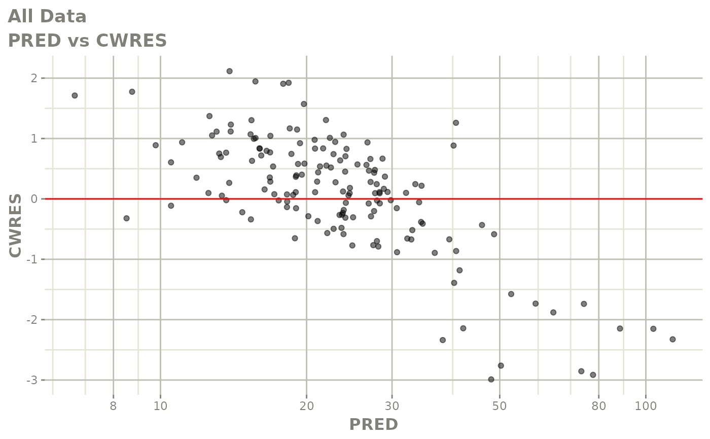
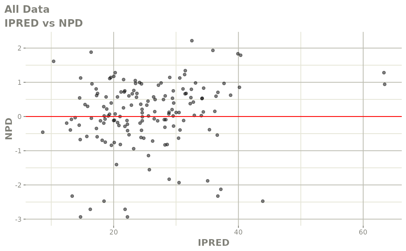
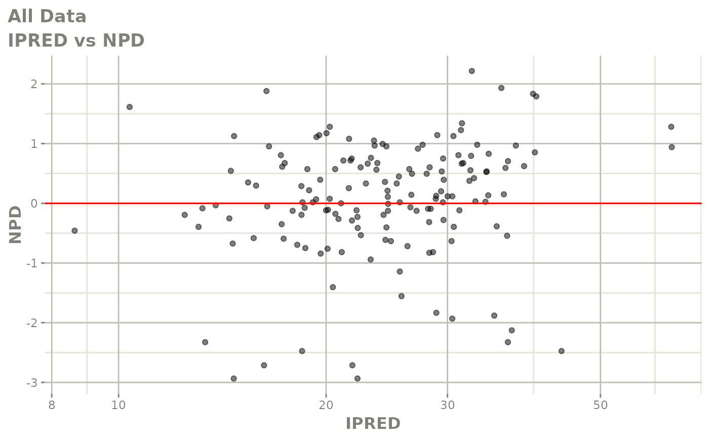
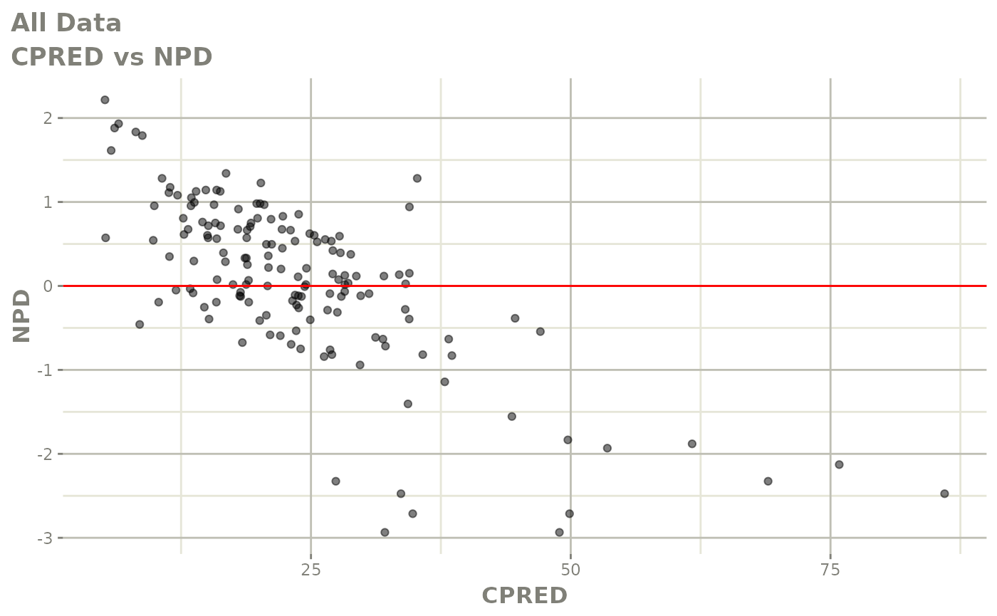
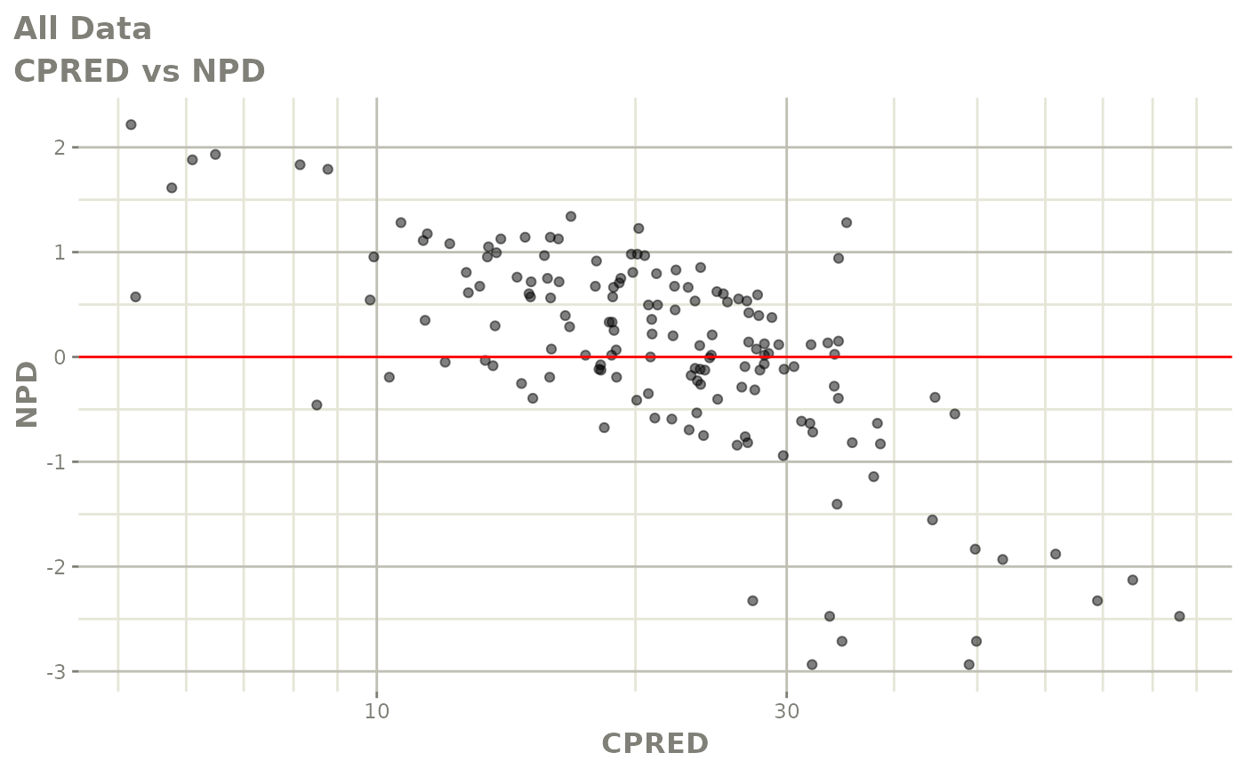
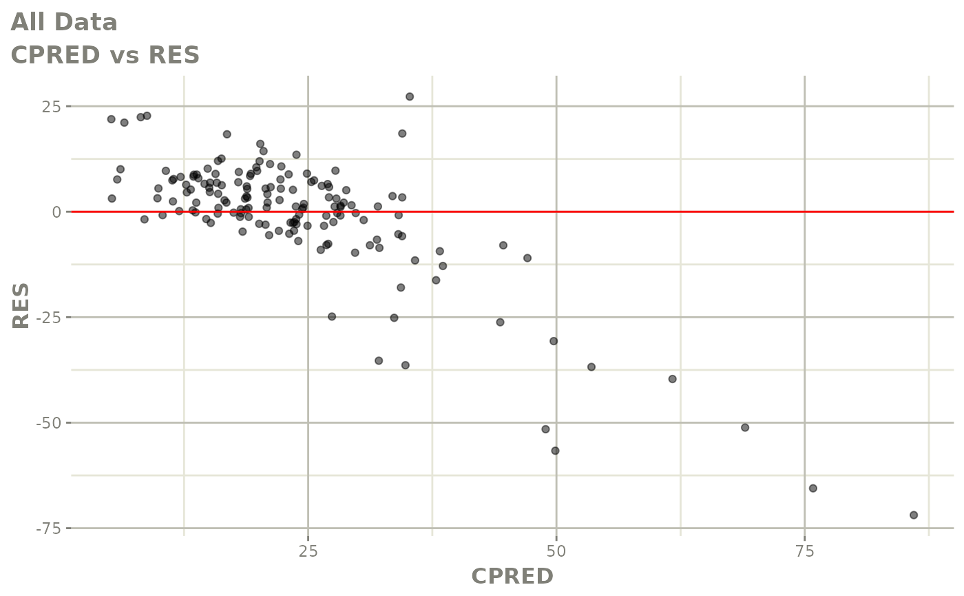
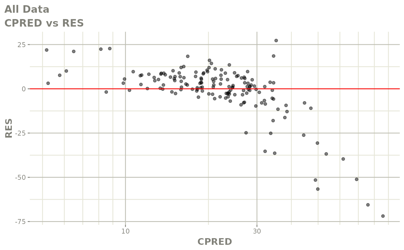
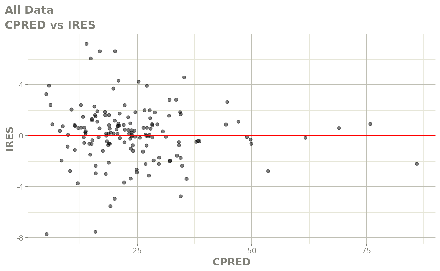
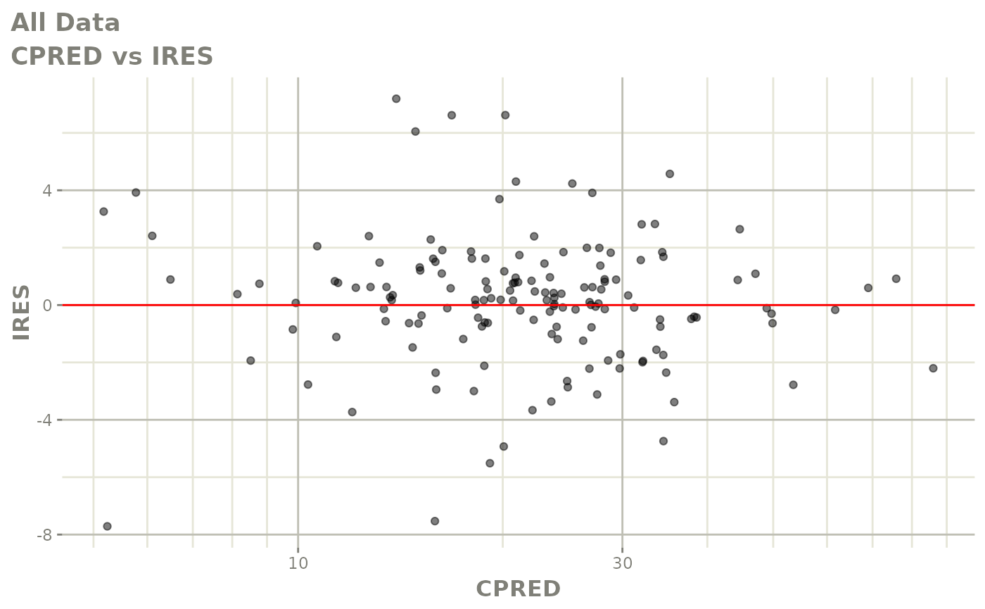
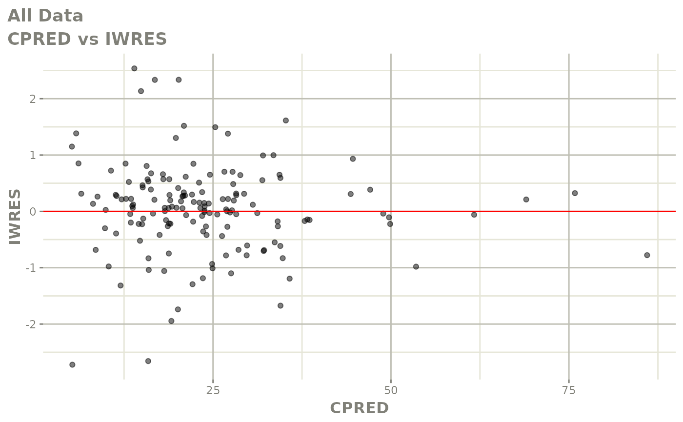
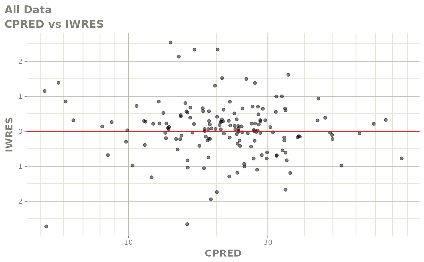
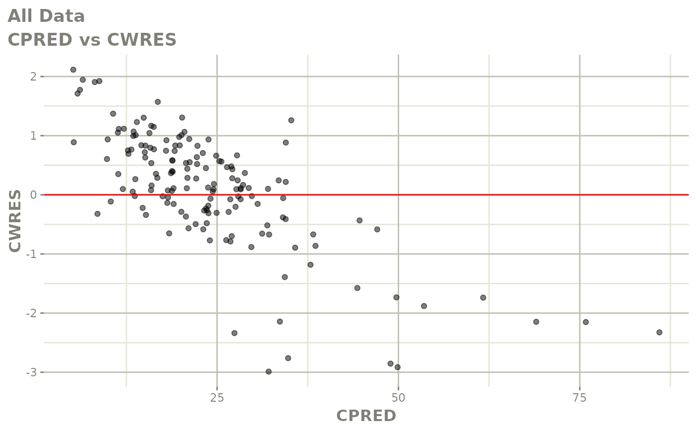
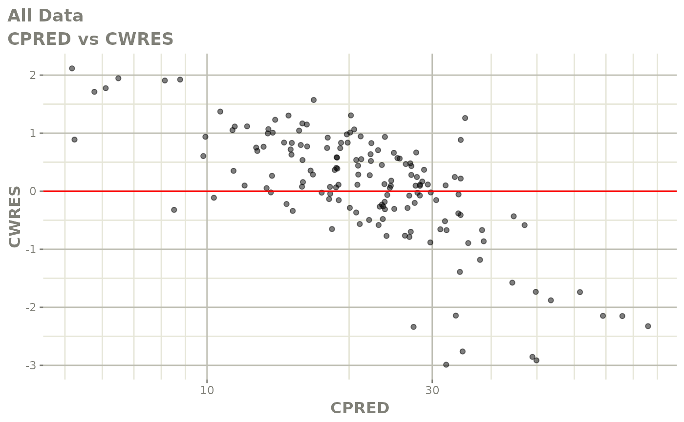
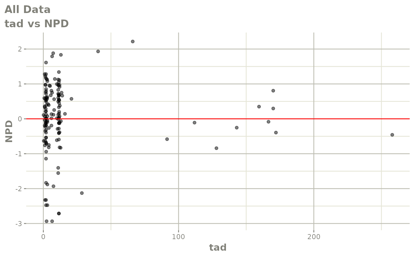
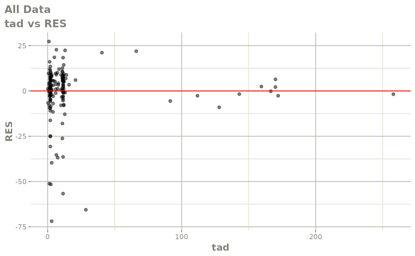
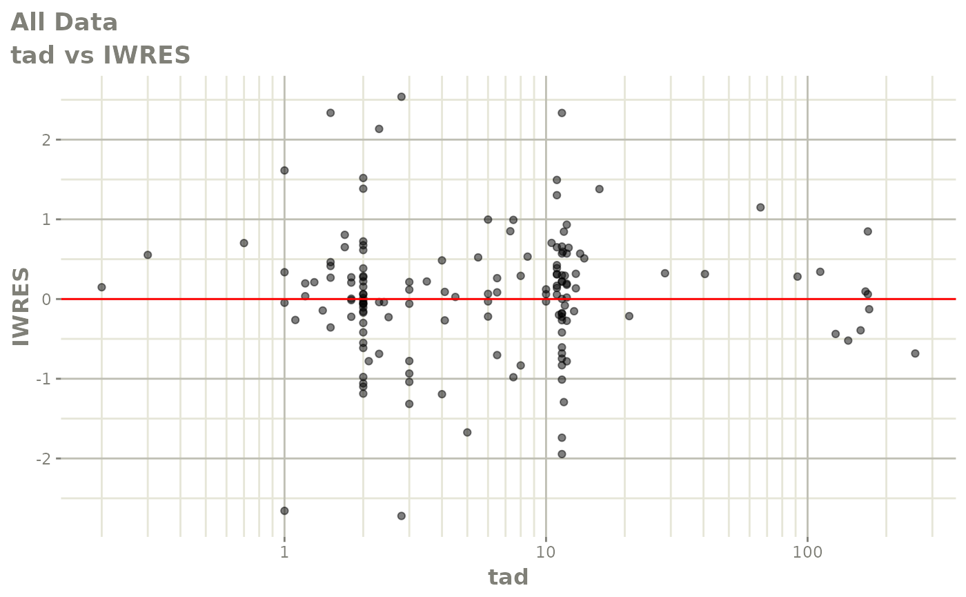
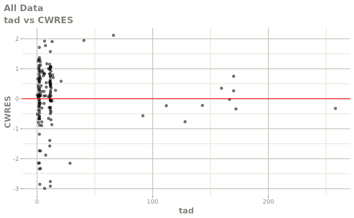
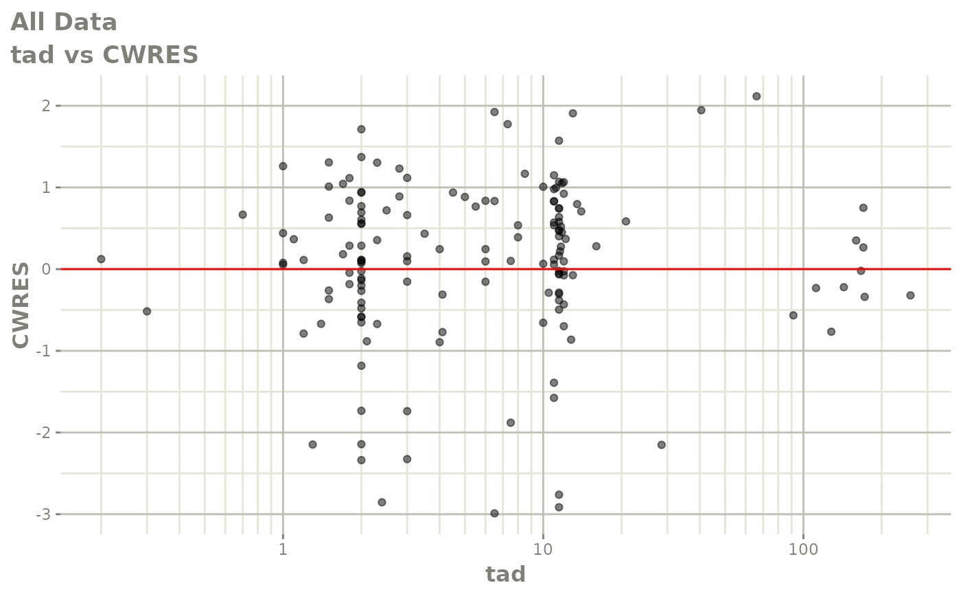
#> # v <dbl>, ke <dbl>, tad <dbl>, dosenum <dbl>Basic Goodness of Fit Plots
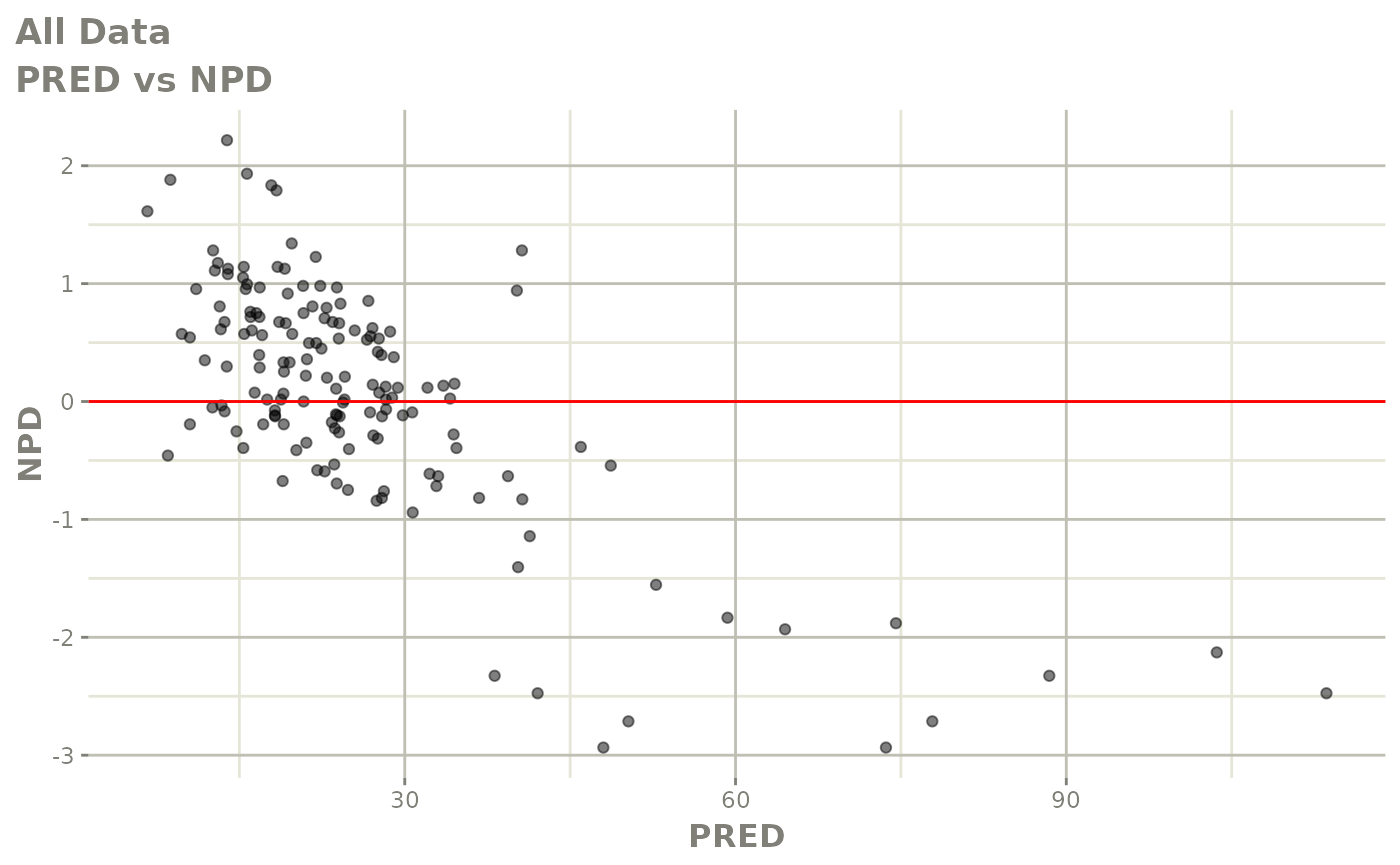
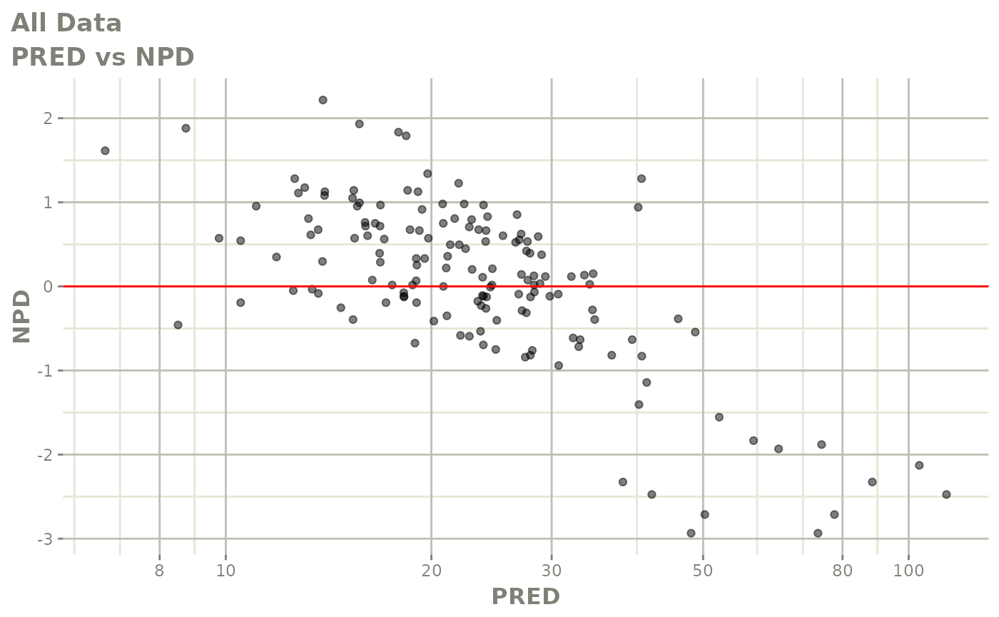
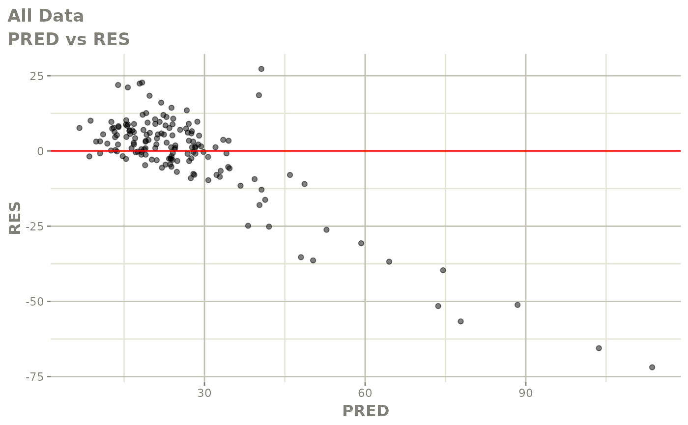
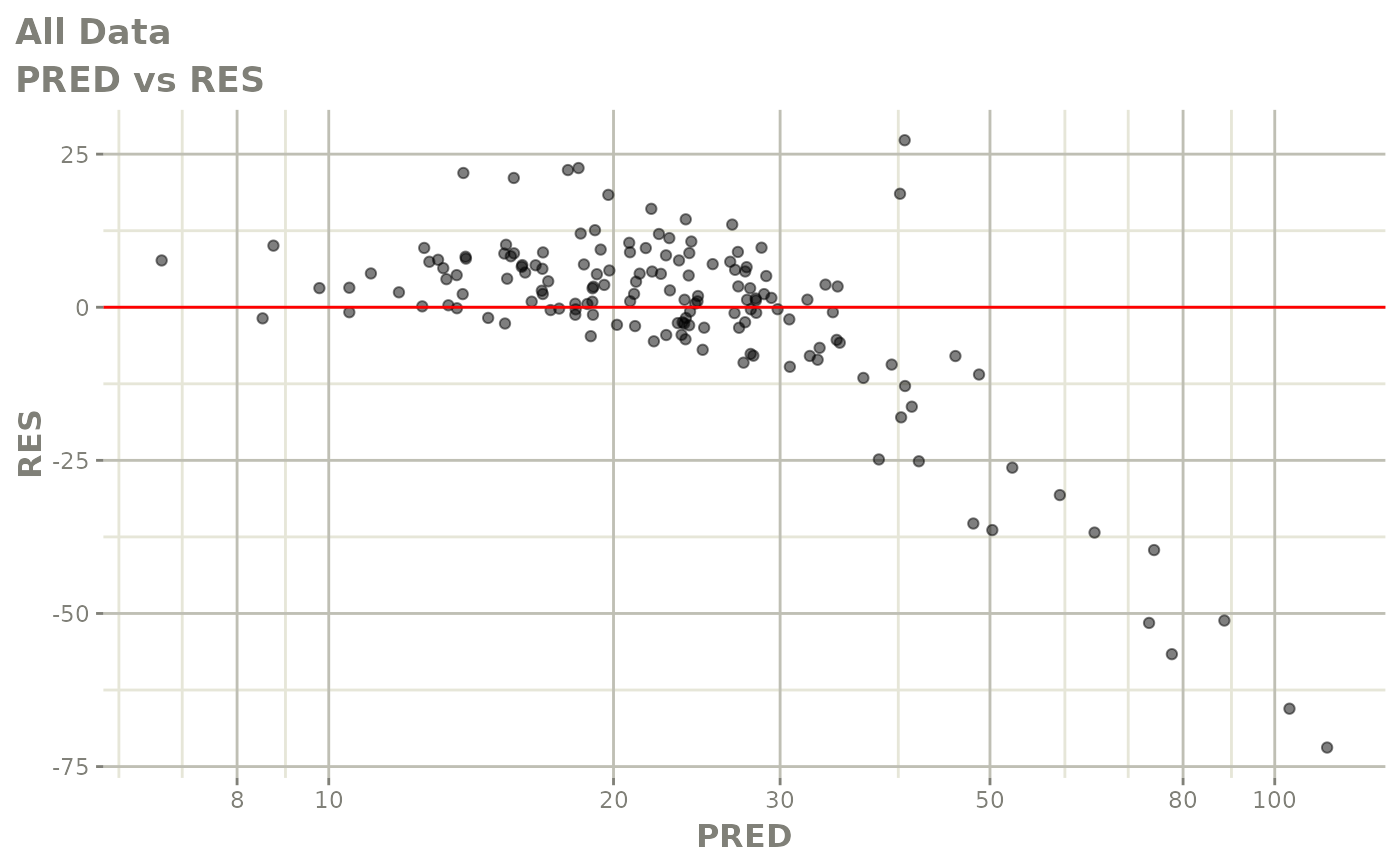
plot(fit)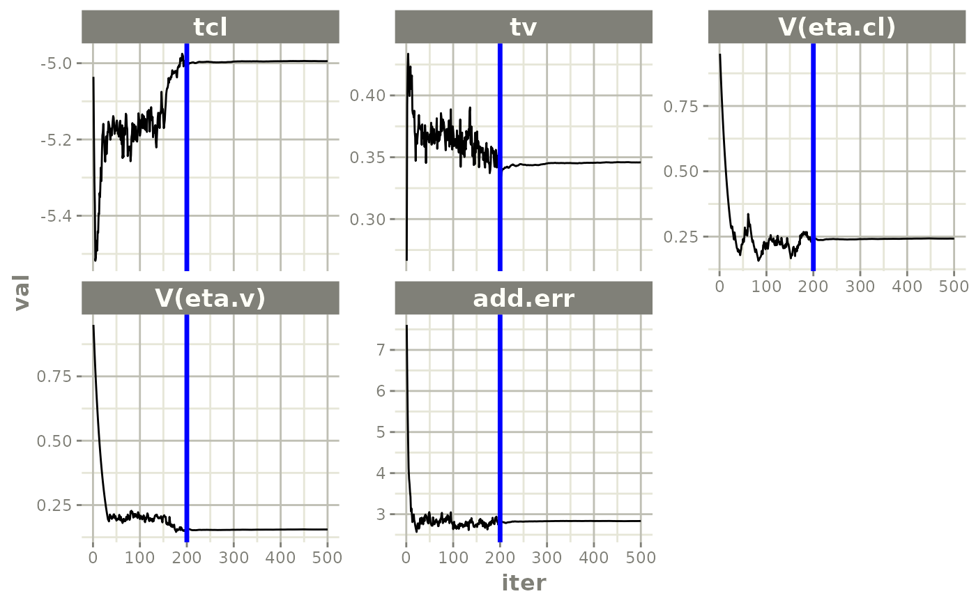
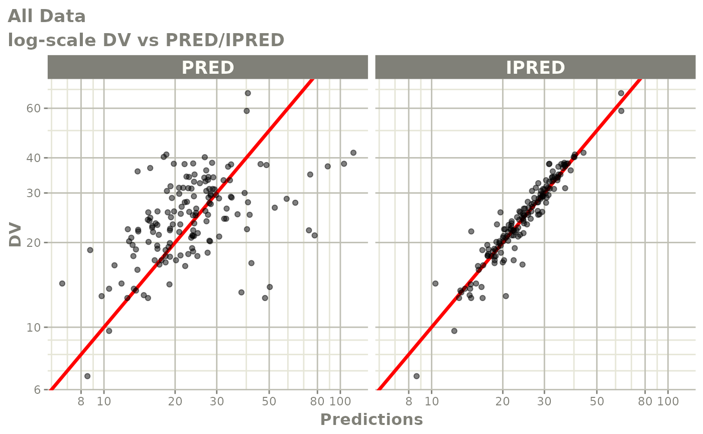
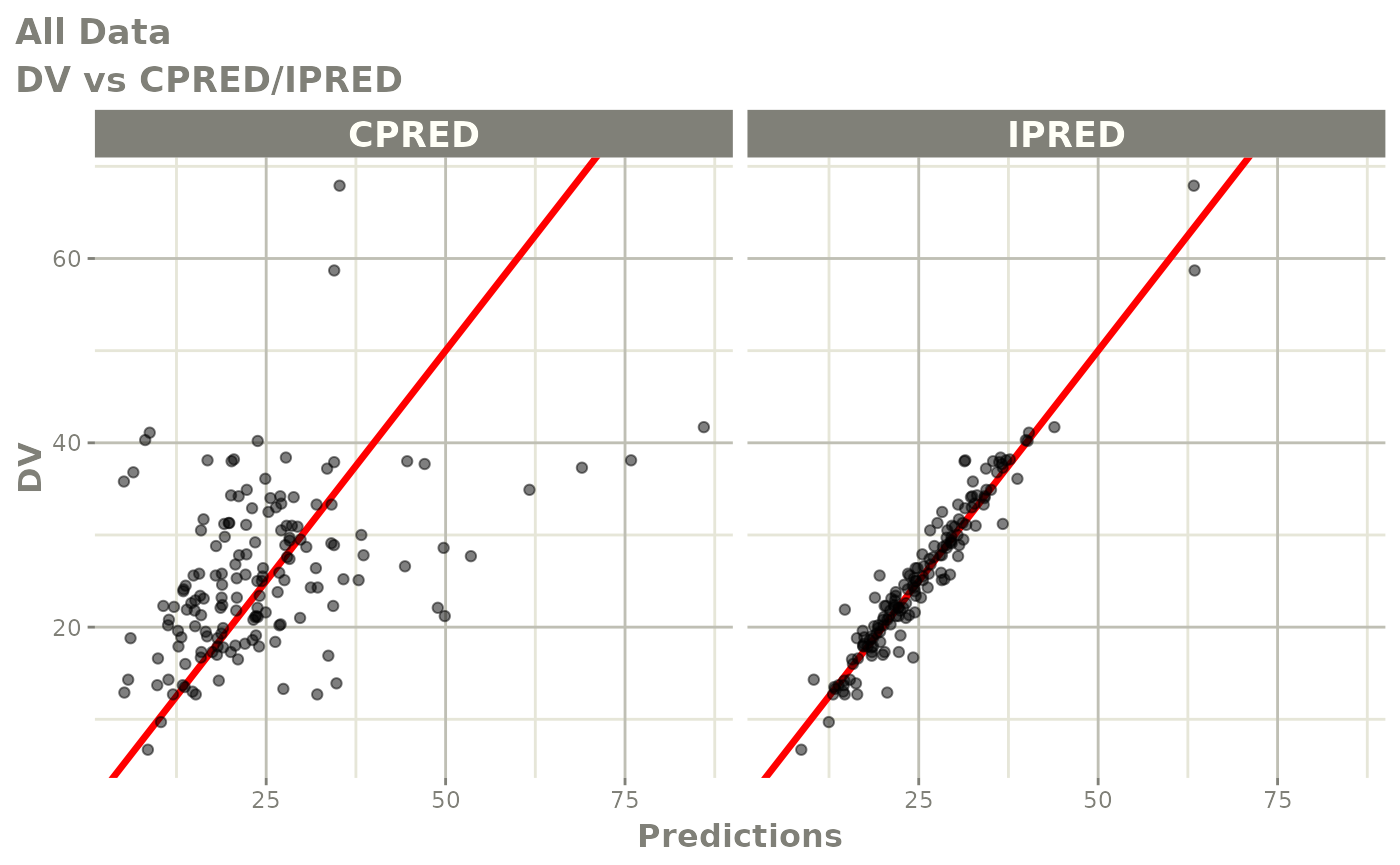
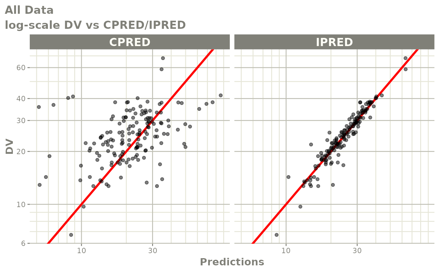
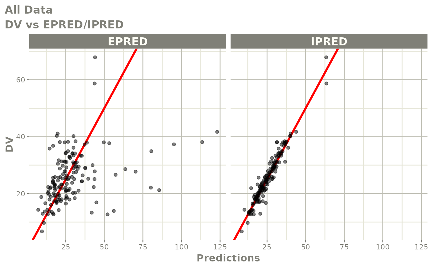

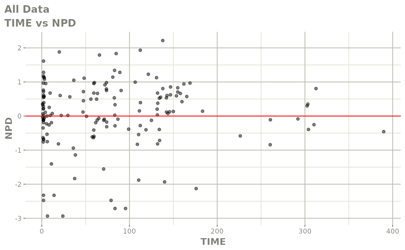
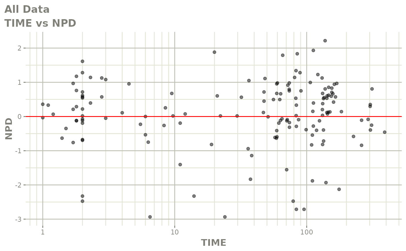
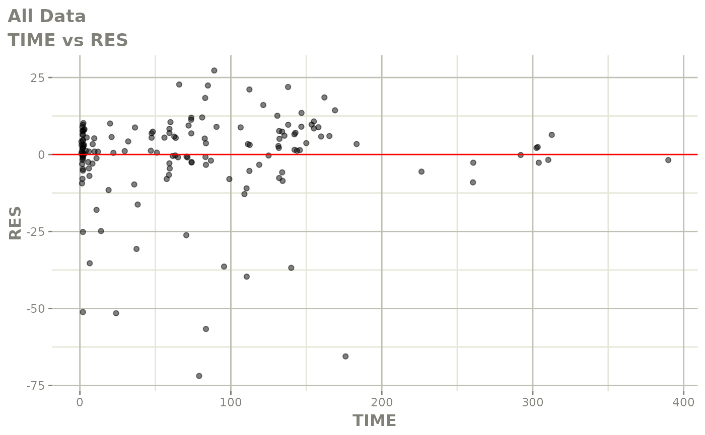
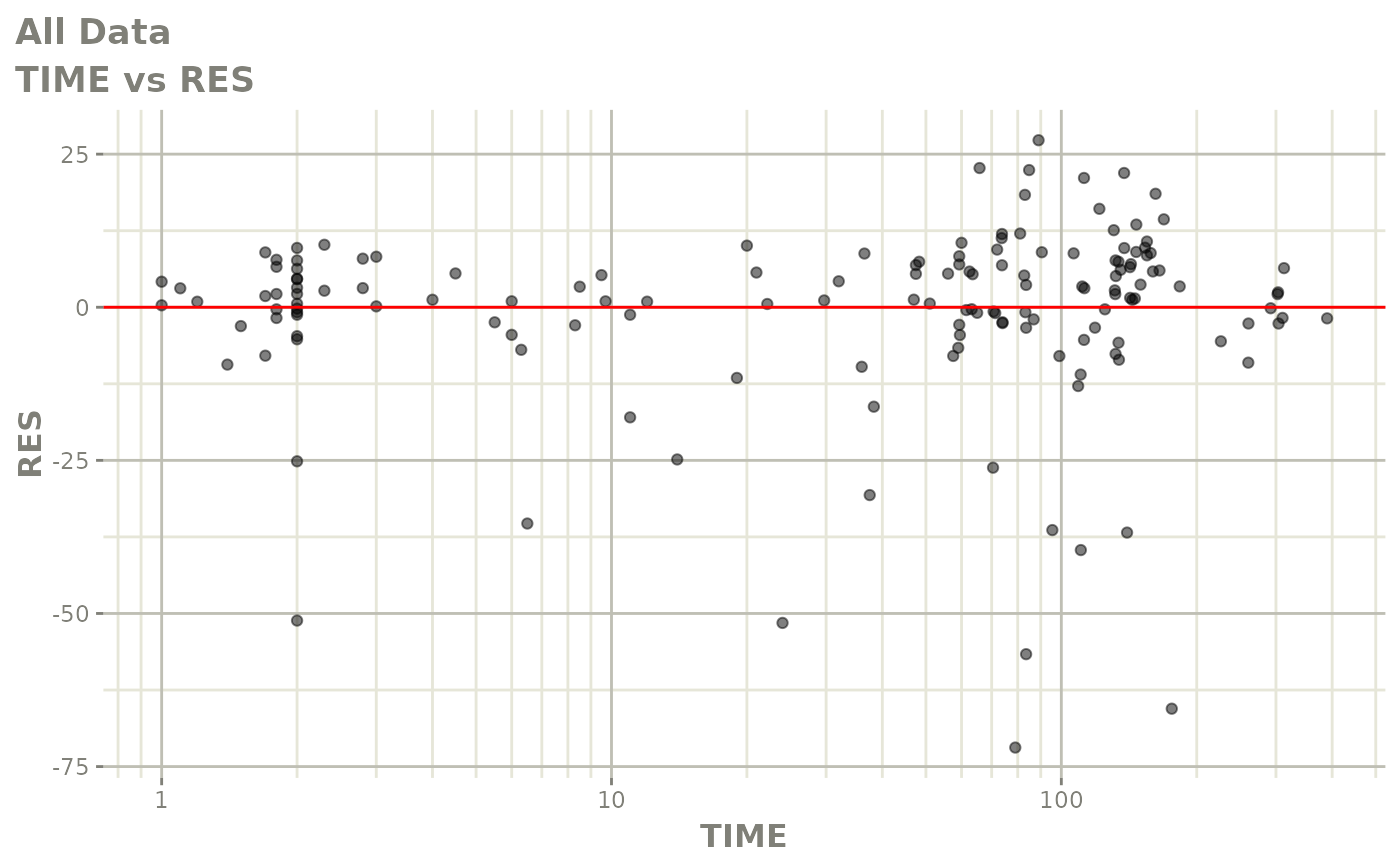
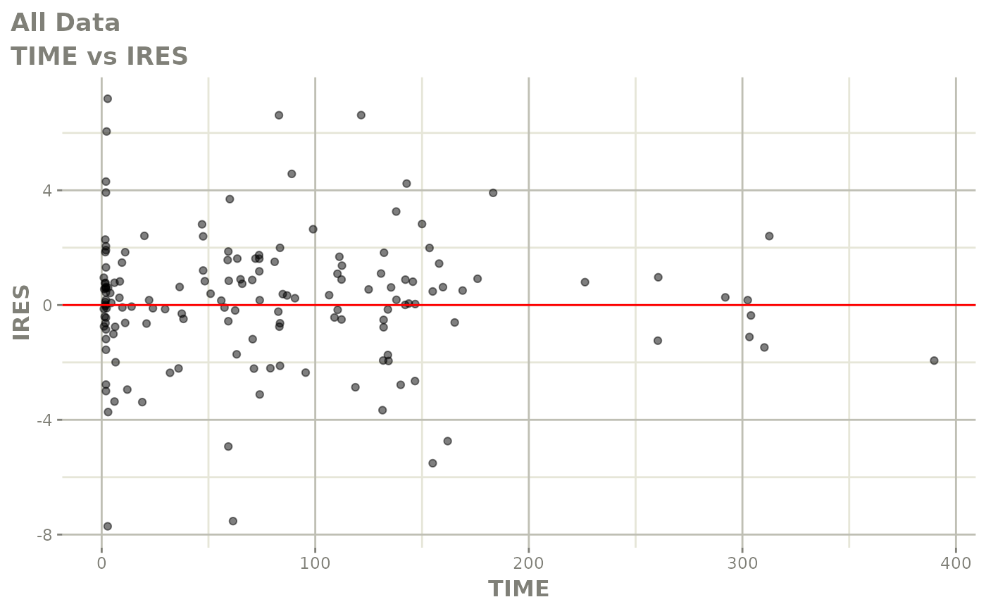
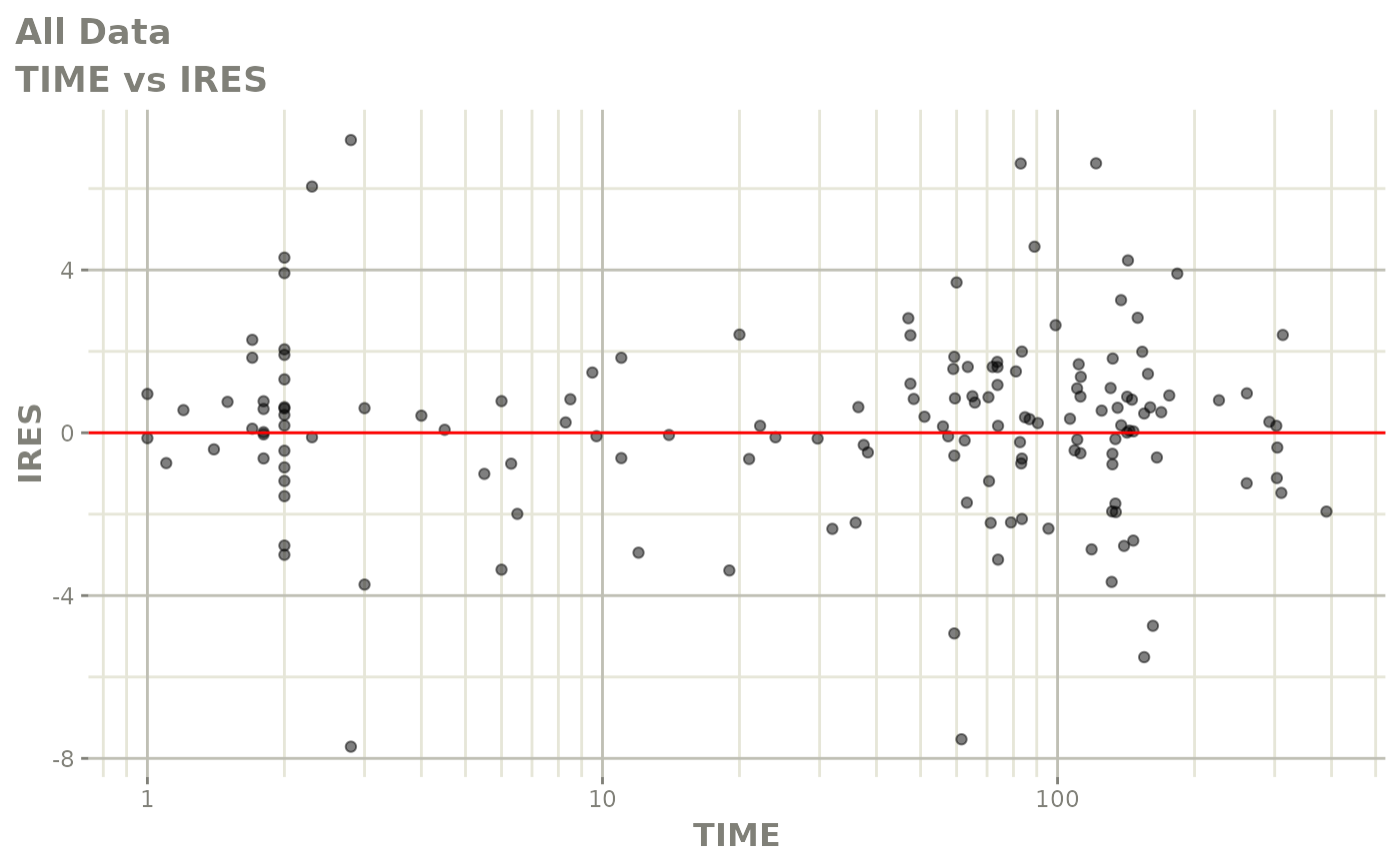
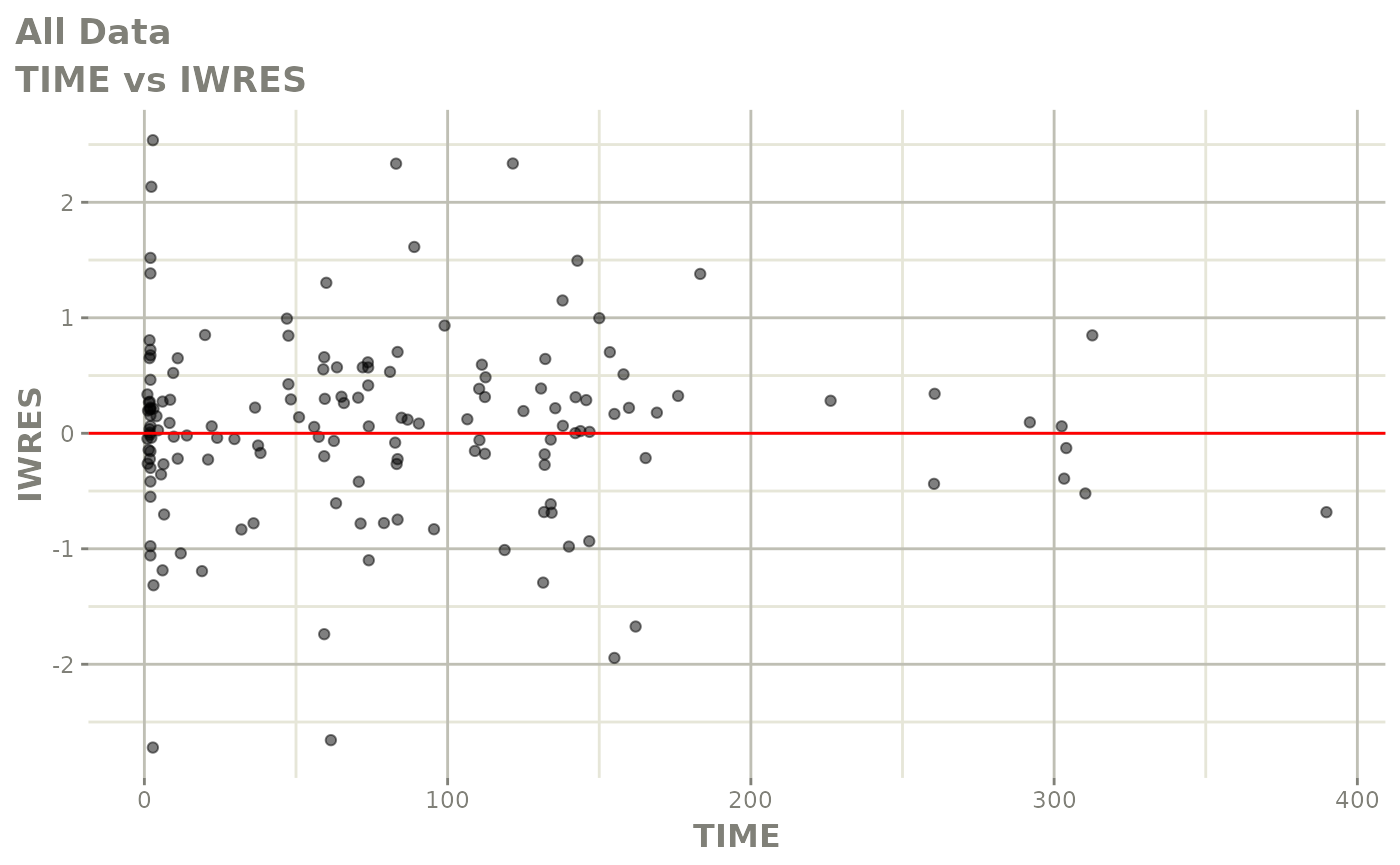
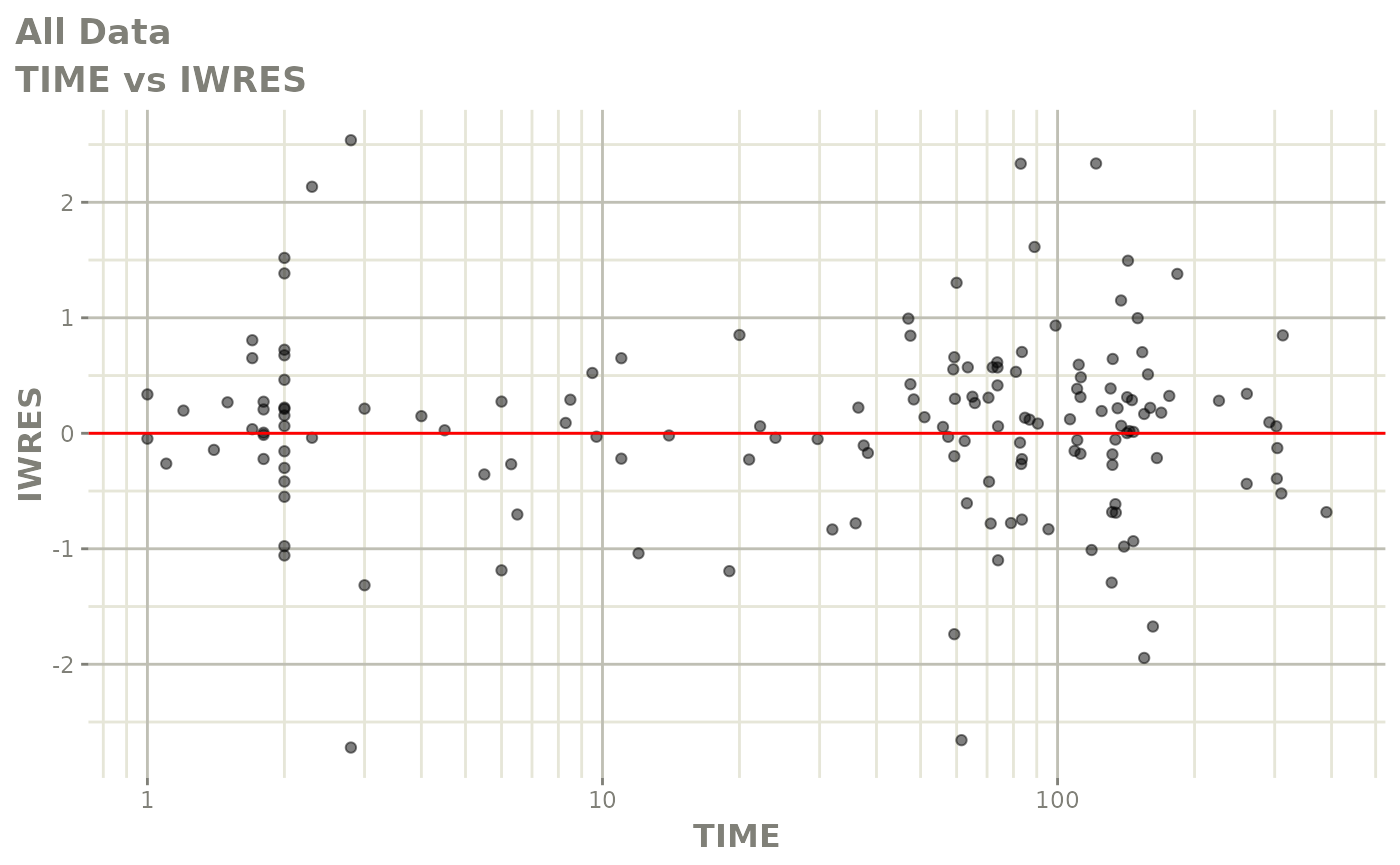
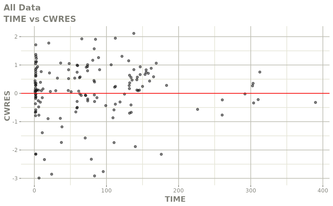


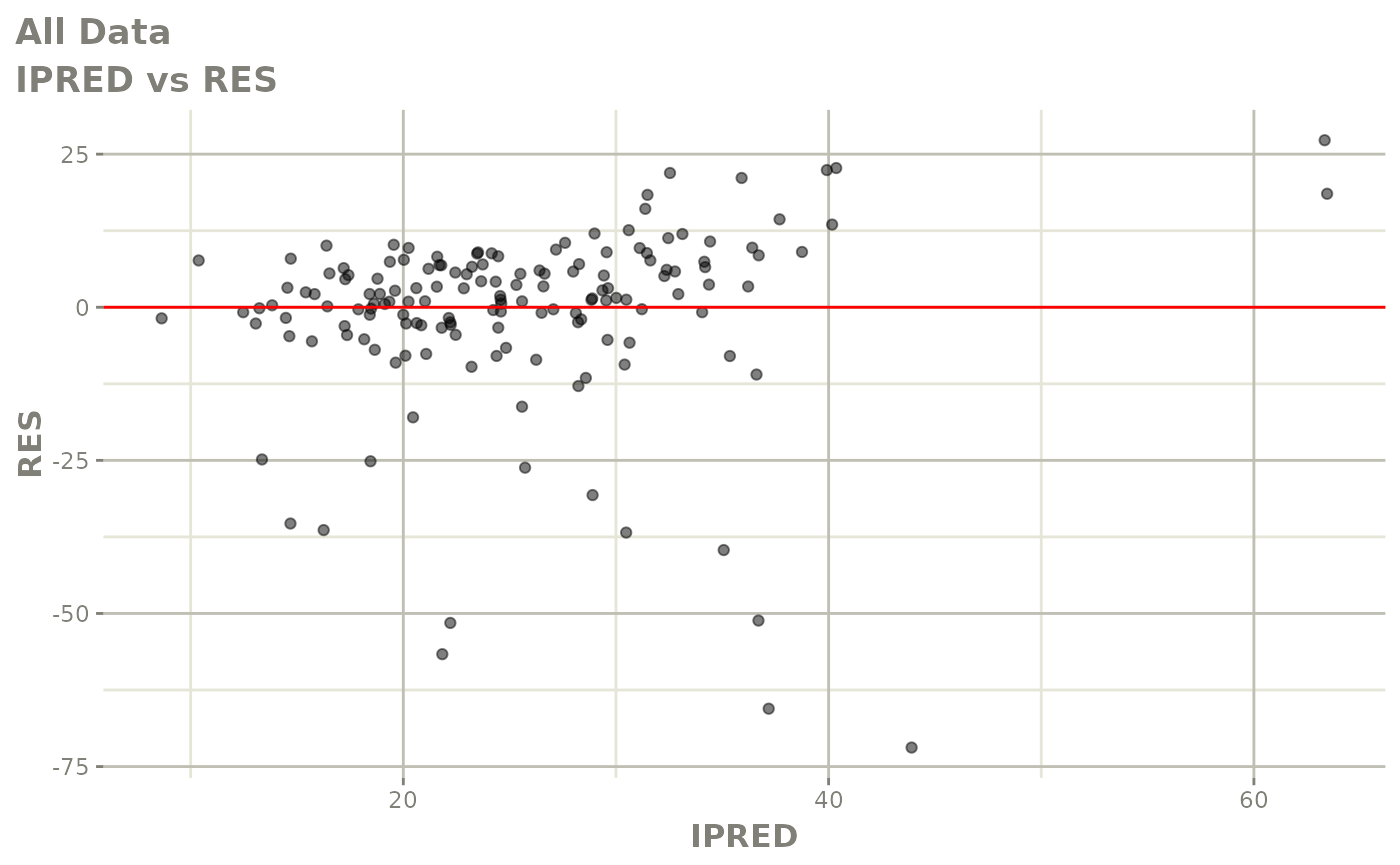
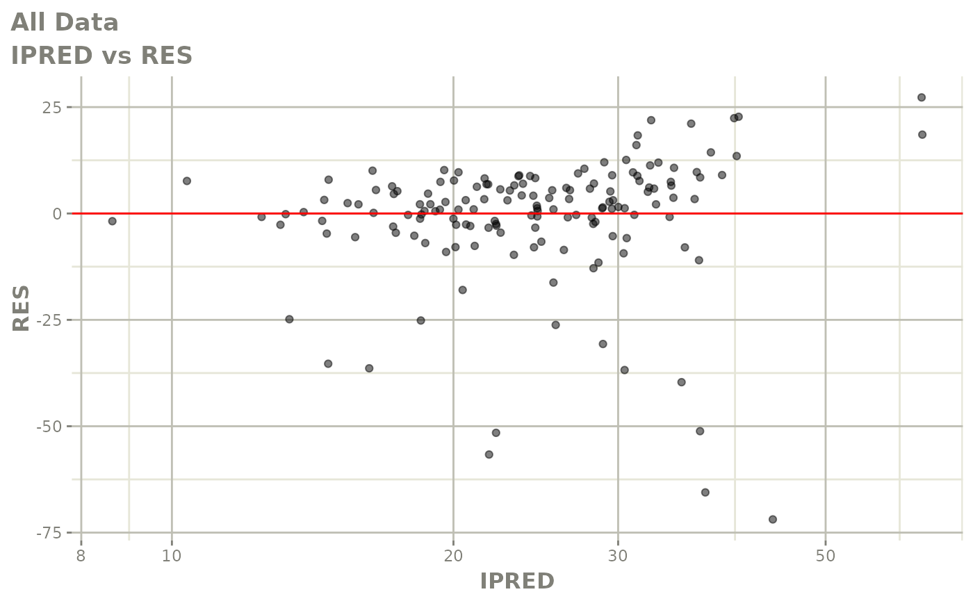
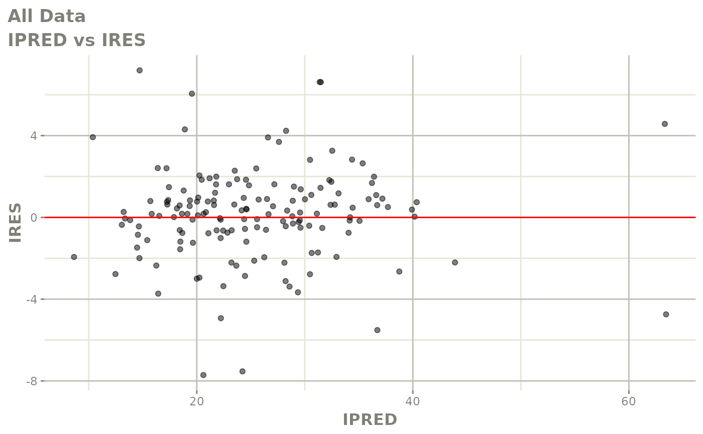
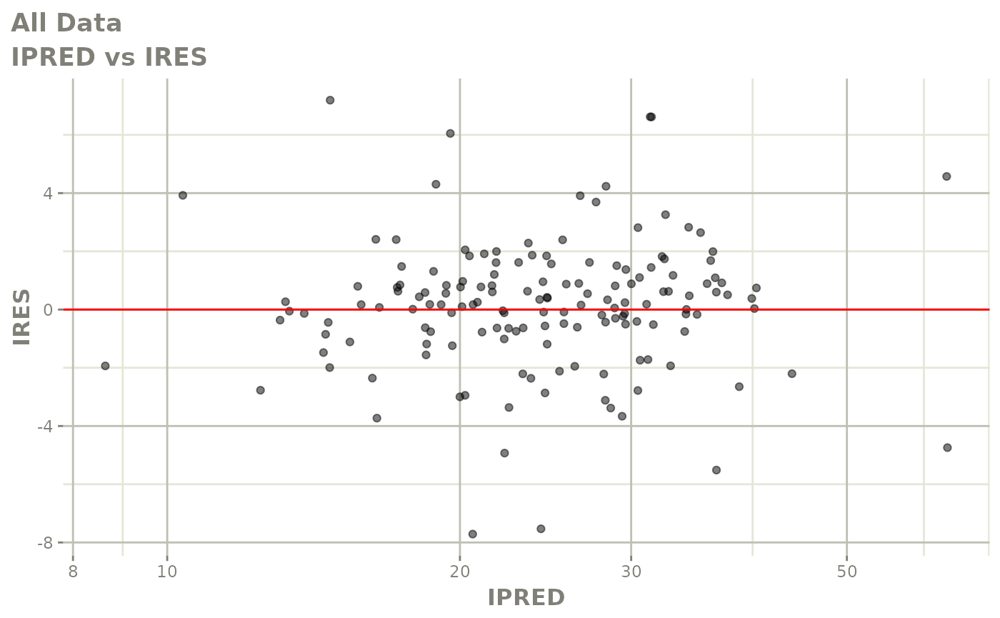
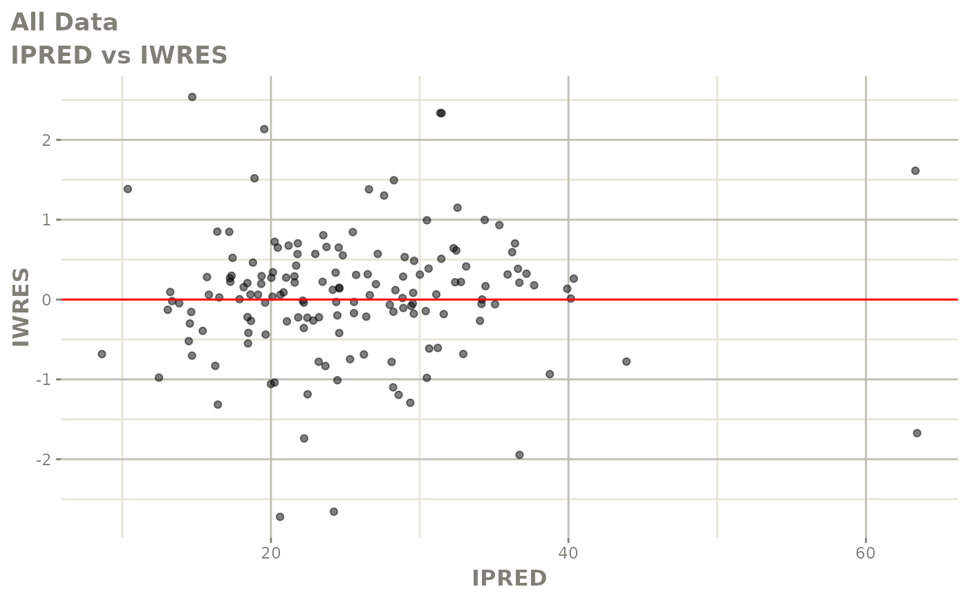
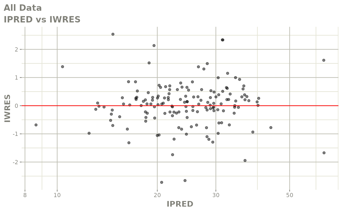
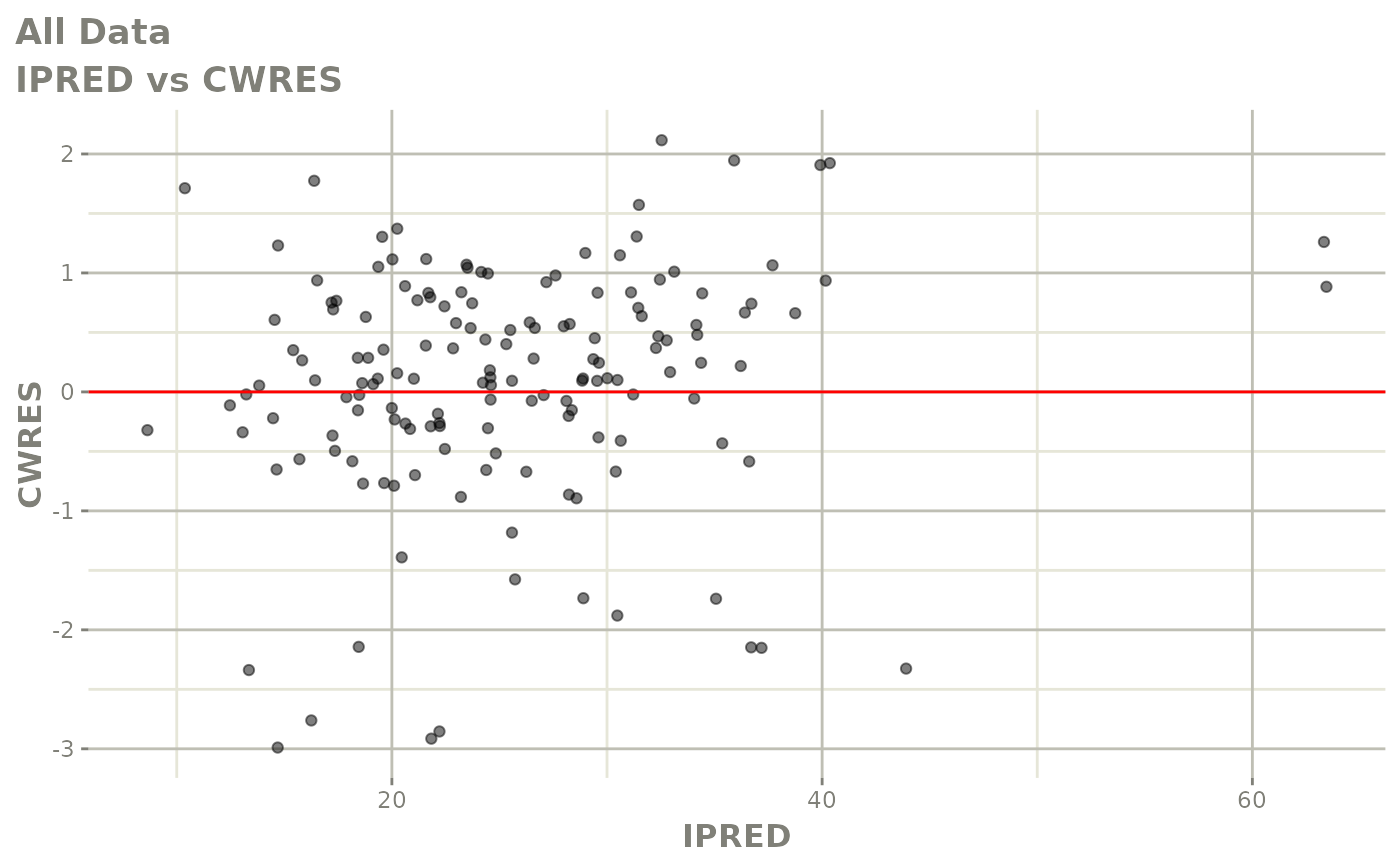
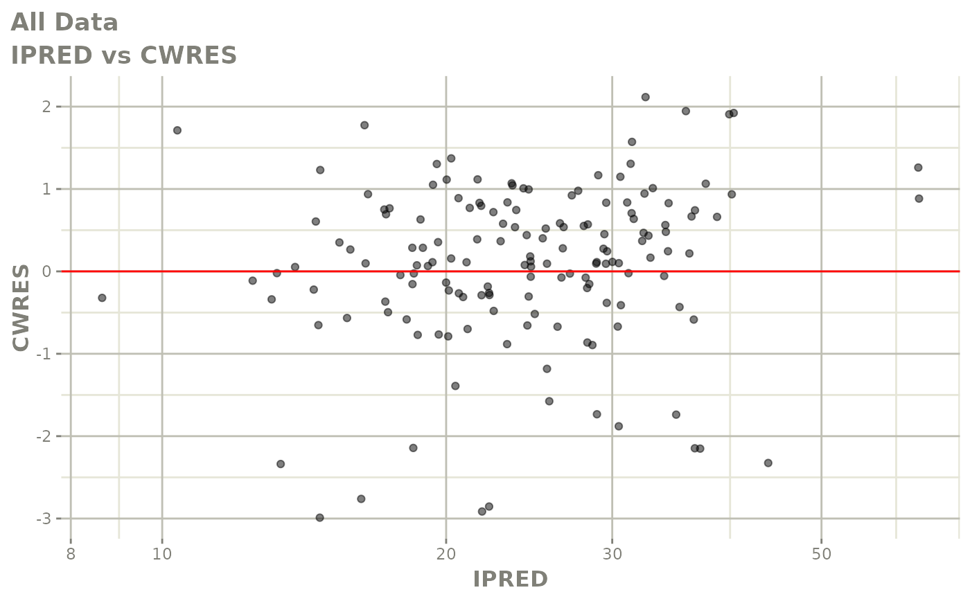

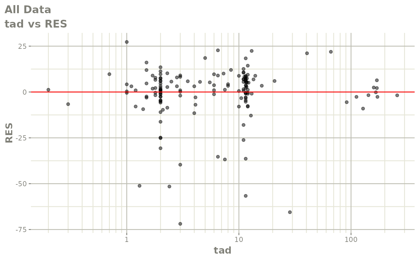
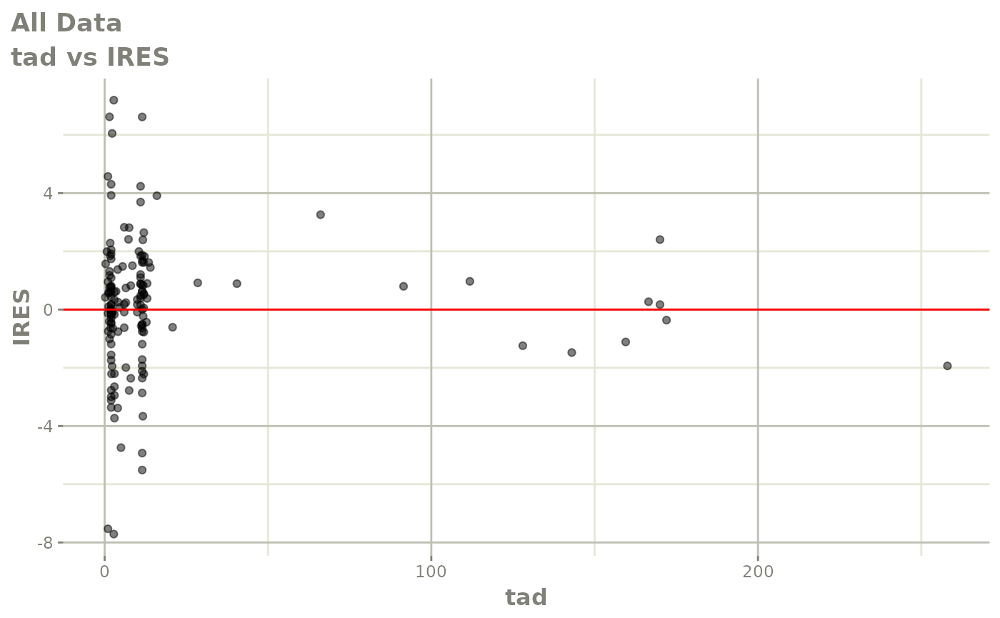
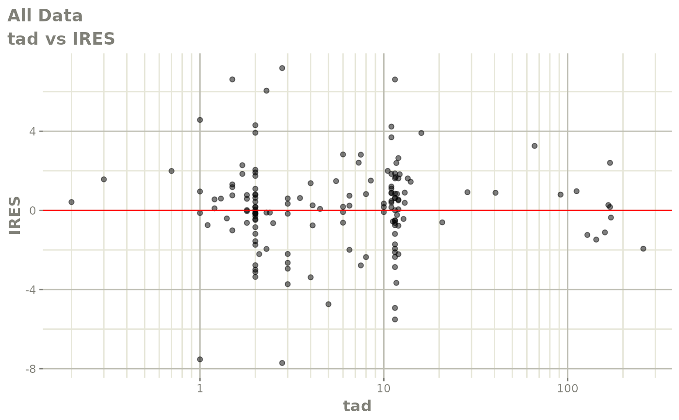
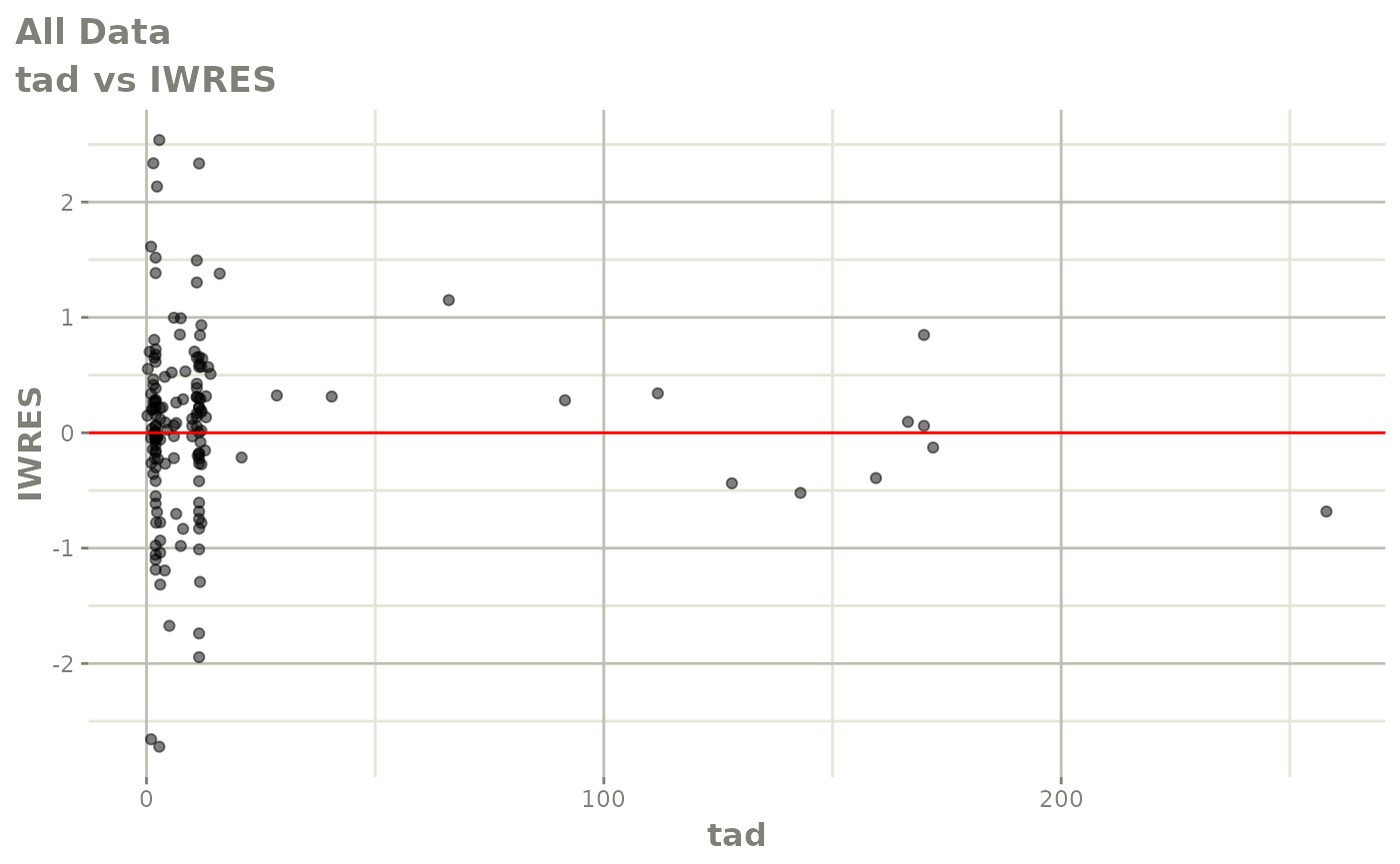
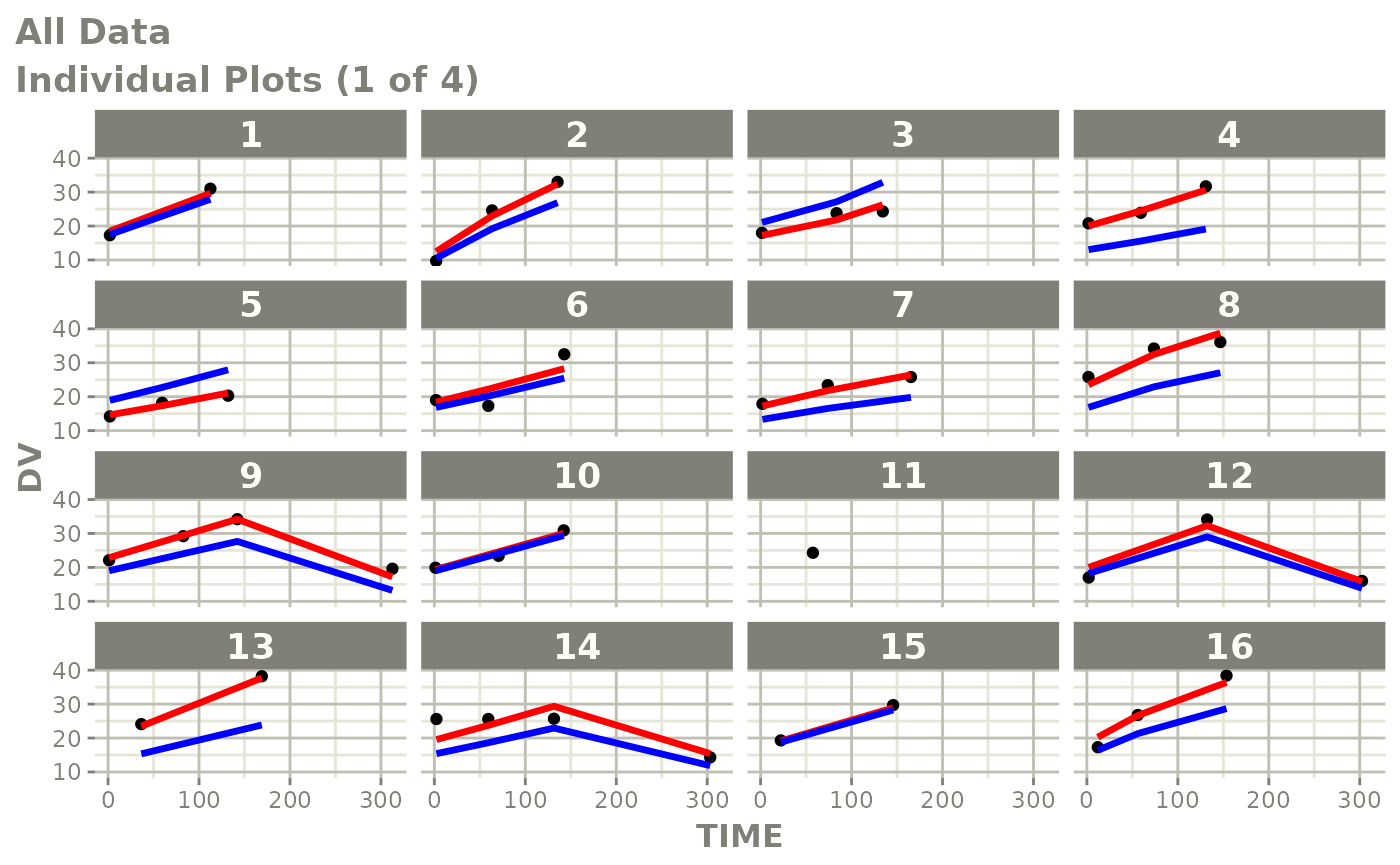
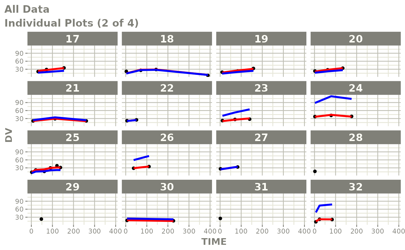
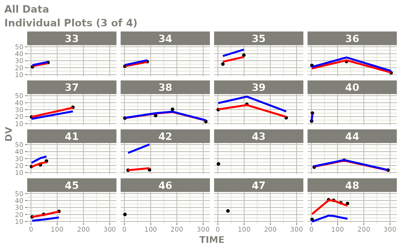
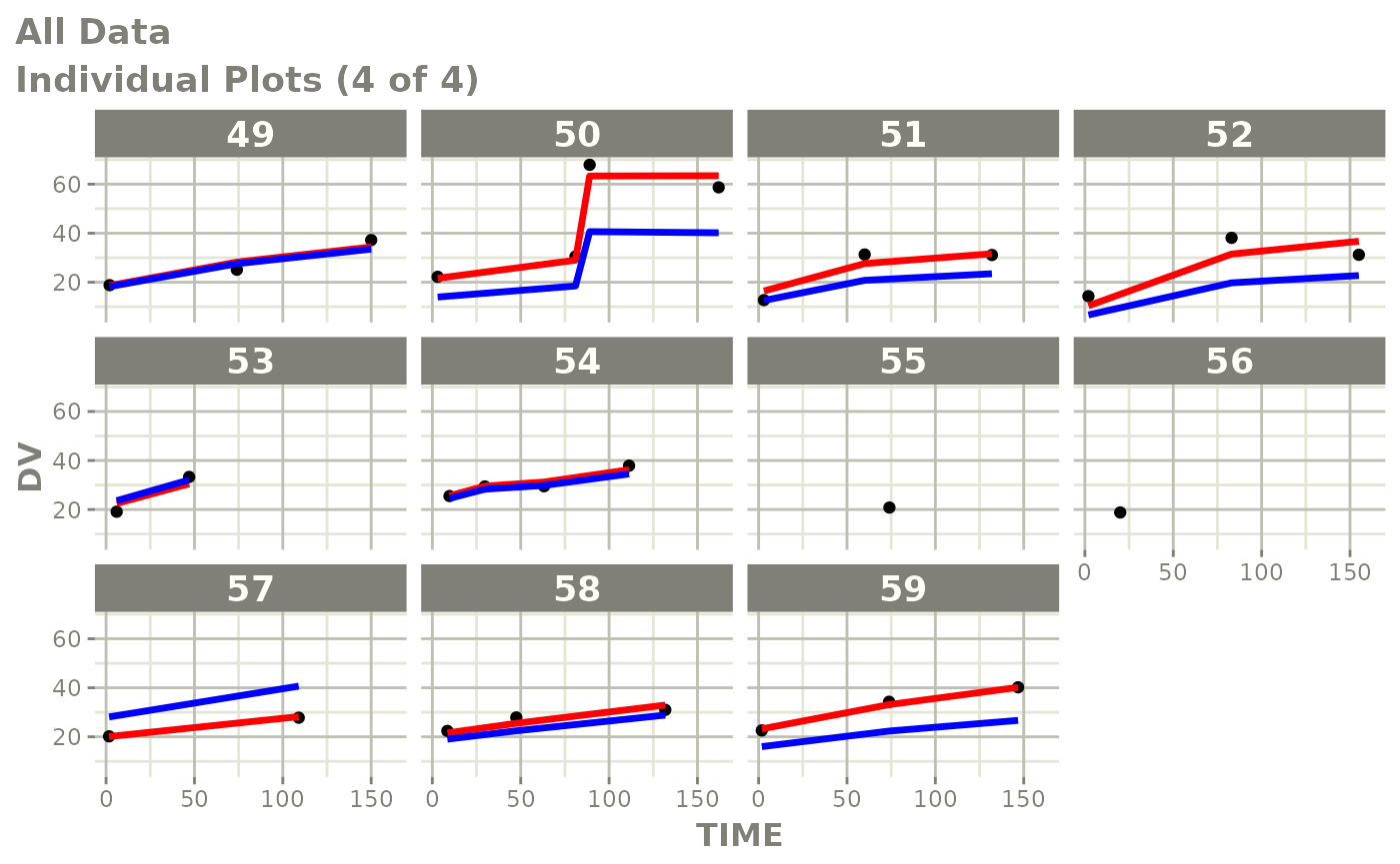
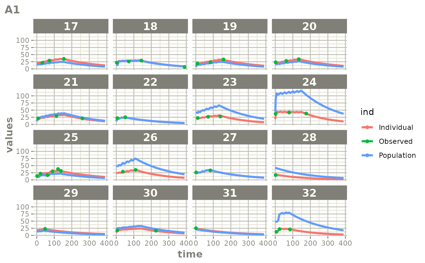
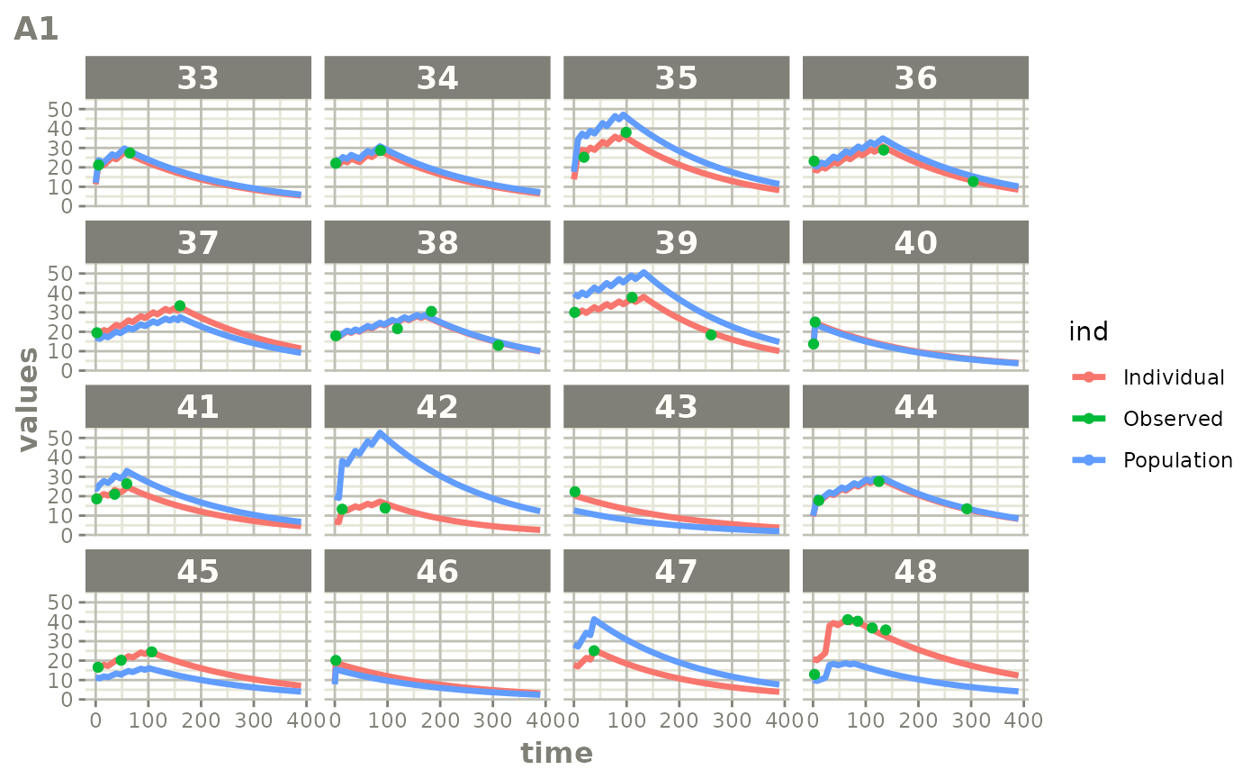
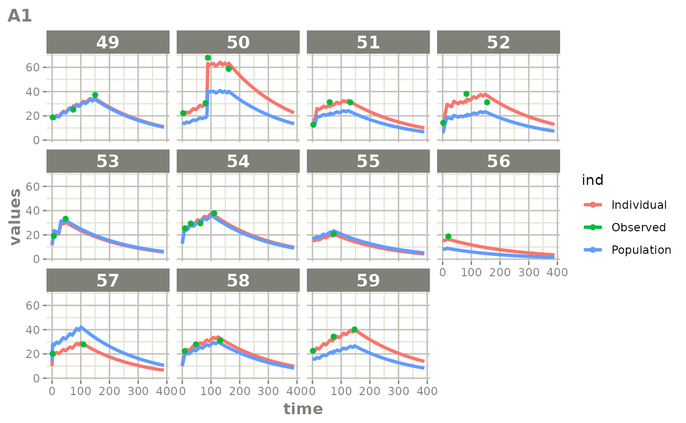
Those individual plots are not that great, it would be better to see
the actual curves; You can with augPred
plot(augPred(fit))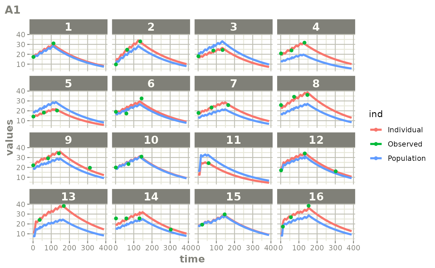
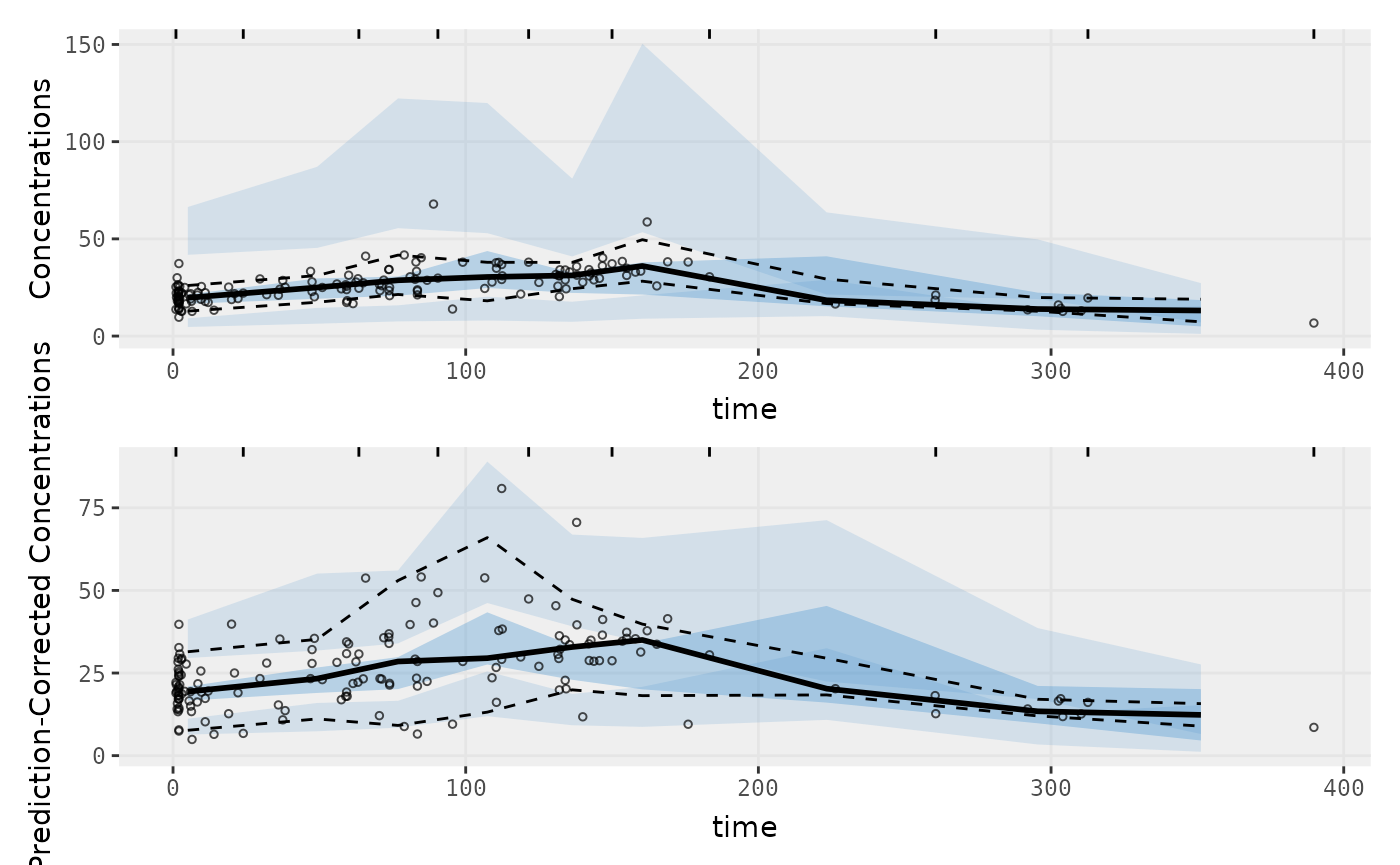
Two types of VPCs
library(ggplot2)
p1 <- vpcPlot(fit, show=list(obs_dv=TRUE));
#> [====|====|====|====|====|====|====|====|====|====] 0:00:00
p1 <- p1 + ylab("Concentrations")

## A prediction-corrected VPC
p2 <- vpcPlot(fit, pred_corr = TRUE, show=list(obs_dv=TRUE))
#> [====|====|====|====|====|====|====|====|====|====] 0:00:00
p2 <- p2 + ylab("Prediction-Corrected Concentrations")

library(patchwork)
p1 / p2