Mixture Models in nlmixr2

Overview

Mixture models describe populations where individuals belong to one of several latent subpopulations, each with distinct fixed-effect parameters. The classic pharmacokinetic example is bimodal clearance due to a polymorphic drug-metabolizing enzyme: extensive metabolizers (EM) clear the drug quickly while poor metabolizers (PM) clear it slowly. A standard single-population model will fit neither group well and will produce inflated between-subject variability for clearance.

nlmixr2est supports mixture models via the mix() function inside the model block. The following estimation methods all support mixture models:

Method	Description
`focei`	First-Order Conditional Estimation with Interaction (recommended)
`foce`	First-Order Conditional Estimation
`fo`	First-Order
`foi`	First-Order with Interaction
`laplace`	Laplace approximation
`agq`	Adaptive Gaussian Quadrature
`saem`	Stochastic Approximation Expectation-Maximization
`imp`	Importance sampling (Monte-Carlo EM)
`impmap`	Importance sampling around the MAP estimate
`qrpem`	Quasi-random parametric EM
`npag`	Nonparametric adaptive grid
`npb`	Nonparametric Bayesian (Dirichlet-process)

Two methods reject a mix() model up front rather than fitting something misleading: emvi and fbvi (mean-field variational inference on the theta-sensitivity model, which has no mixture structure) stop with cannot have a mixture model (ie 'mix()') for the estimation routine. vae does not currently fit a mixture model either.

The gradient-based methods (focei, foce, fo, foi, laplace, agq) all use the same hard-assignment strategy described below and reliably separate mixture components with high precision. SAEM’s mixture machinery is a soft-assignment (EM responsibility) scheme, described in its own section, Mixture Models with SAEM — though its default, mixProbMethod = "regress", hard-classifies each subject once and skips the per-iteration responsibility step, which is what makes the default immune to the mixing-probability collapse that scheme is otherwise prone to. Even so, on small or weakly-separated datasets it may separate components less precisely than the gradient-based methods. focei is recommended when precise per-subject classification matters; SAEM is a usable alternative that may need tuning (see its section) to match it. The EM/sampling and nonparametric families are covered in Other estimation families.

rxode2 requirements. Nested transformations inside mix() — for example mix(expit(tcl1 + eta.cl, 0.1, 200), p1, ...) — require rxode2 >= 5.1.3. Earlier versions translate only the top-level mix() arguments and will silently mis-handle the inner expit()/logit()/exp() calls.

Reading mixest/mixnum back out of the fitted table (see Reading the component off the fit table) additionally requires an rxode2 carrying the fix in nlmixr2/rxode2#1358, which is newer than 5.1.7. This was a bug, not a design limit: up to that version the prediction model lost its mix() call to symengine and rxode2 no longer read it as a mixture, so those columns — and every model variable computed from mix() — came back as 0 for every row, with PRED/IPRED computed from those zeros. You do not have to check the version: a fit on an affected rxode2 now says so in $runInfo ("mixture not passed to table; mixest/mixnum read 0"). The parameter estimates, $mixNum and $mixList were never affected — the bug was confined to the table.

Motivating Example: Bimodal Clearance

To illustrate the approach we simulate a 30-subject study with two distinct clearance populations — roughly mimicking a drug whose metabolism is governed by a CYP2D6 polymorphism.

library(nlmixr2est)
library(rxode2)

set.seed(2024)

# True population parameters
tclEm   <- log(8)    # fast metabolizers (EM), CL = 8 L/hr
tclPm   <- log(0.8)  # slow metabolizers (PM), CL = 0.8 L/hr  (10× lower)
tv      <- log(30)   # volume of distribution
tka     <- log(1.2)  # absorption rate constant
sigma   <- 0.20      # proportional residual SD
omegaCl <- 0.09      # BSV on CL (variance)
omegaV  <- 0.04      # BSV on V

nEm <- 20            # 67% extensive metabolizers
nPm <- 10            # 33% poor metabolizers
n   <- nEm + nPm

# Simulate per-subject parameters
clTrue <- c(
  exp(tclEm + rnorm(nEm, 0, sqrt(omegaCl))),
  exp(tclPm + rnorm(nPm, 0, sqrt(omegaCl)))
)
vTrue  <- exp(tv + rnorm(n, 0, sqrt(omegaV)))
kaTrue <- rep(exp(tka), n)
group  <- rep(c("EM (fast)", "PM (slow)"), c(nEm, nPm))

# Observation times
times <- c(0.5, 1, 2, 4, 6, 8, 12, 18, 24, 36, 48)

# One-compartment oral model
modSim <- rxode2({
  d/dt(depot)   <- -ka * depot
  d/dt(central) <- ka * depot - (cl / v) * central
  cp <- central / v
})

simRows <- vector("list", n)
for (i in seq_len(n)) {
  ev  <- et(amt = 100, time = 0) |> et(time = times)
  out <- rxSolve(modSim,
                 params = c(ka = kaTrue[i], cl = clTrue[i], v = vTrue[i]),
                 events = ev)
  dv  <- out$cp * exp(rnorm(length(times), 0, sigma))
  simRows[[i]] <- data.frame(
    ID    = i,
    time  = times,
    DV    = pmax(dv, 1e-6),
    group = group[i],
    AMT   = 0,
    EVID  = 0
  )
}

# Add dosing rows (EVID=1)
doseRows <- data.frame(
  ID = seq_len(n), time = 0, DV = NA_real_,
  group = group, AMT = 100, EVID = 1
)
simData <- rbind(doseRows, do.call(rbind, simRows))
simData <- simData[order(simData$ID, simData$time), ]

Why a standard model fails

Plotting the raw concentration–time profiles immediately reveals the bimodality:

obs <- simData[simData$EVID == 0, ]

# manual colour palette — no external packages needed
cols <- c("EM (fast)" = "#2166AC", "PM (slow)" = "#D6604D")

plot(NA, xlim = c(0, 48), ylim = c(0, max(obs$DV) * 1.05),
     xlab = "Time (hr)", ylab = "Concentration",
     main = "Observed profiles by true metabolizer status")
for (grp in c("EM (fast)", "PM (slow)")) {
  sub <- obs[obs$group == grp, ]
  for (id in unique(sub$ID)) {
    d <- sub[sub$ID == id, ]
    lines(d$time, d$DV, col = cols[grp], lwd = 1.2)
  }
}
legend("topright", legend = names(cols), col = cols, lwd = 2, bty = "n")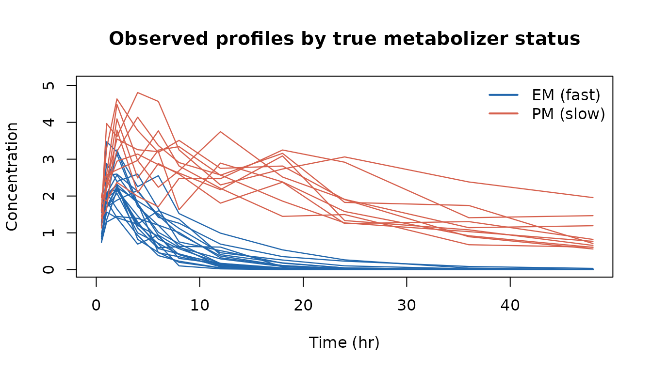

Simulated PK profiles coloured by true metabolizer status. The 10-fold difference in clearance creates two non-overlapping trajectory bundles — a standard single-population model cannot capture this structure.

The two bundles of trajectories are separated by roughly an order of magnitude in exposure — exactly the situation where a mixture model should be used.

Model Specification

Mixture models are declared with mix(expr1, prob1, expr2, ...):

expr1, expr2, … are the parameter expressions for each component
prob1 is the prior mixing probability for the first component; the last component’s probability is implicit (1 - prob1)
One fewer probability parameter than components is required

twoPop <- function() {
  ini({
    tka   <- log(1.2)                   # log Ka
    tcl1  <- logit(0.8, 0.1, 200)      # log Cl, EM subpopulation
    tcl2  <- logit(0.8, 0.1, 200)      # log Cl, PM subpopulation
    tv    <- log(30)                     # log V
    p1    <- 0.67                        # prior prob of being an EM
    eta.cl ~ 0.09
    eta.v  ~ 0.04
    add.sd <- 0.2
  })
  model({
    ka <- exp(tka)
    cl <- mix(expit(tcl1 + eta.cl, 0.1, 200), p1, expit(tcl2 + eta.cl, 0.1, 200))
    v  <- exp(tv + eta.v)
    linCmt() ~ add(add.sd)
  })
}

Fitting

fit := nlmixr2(twoPop, simData, "focei",
               control = foceiControl(print = 0))
print(fit)
#> ── nlmixr² FOCEi (outer: bobyqa) ──
#> 
#>            OBJF      AIC      BIC Log-likelihood Condition#(Cov)
#> FOCEi -262.1474 360.3521 390.7448       -172.176        2020.141
#>       Condition#(Cor)
#> FOCEi         55.8794
#> 
#> ── Time (sec $time): ──
#> 
#>            setup optimize covariance preprocess postprocess table compress
#> elapsed 2.574444 1.071376  0.8652653      0.051        0.05  0.08    0.007
#>             other
#> elapsed 0.6319146
#> 
#> ── Population Parameters ($parFixed or $parFixedDf): ──
#> 
#>         Est.     SE %RSE Back-transformed(95%CI) BSV(CV% or SD) Shrink(SD)%
#> tka    0.169 0.0476 28.1       1.18 (1.08, 1.30)                           
#> tcl1   -3.32 0.0843 2.54       7.06 (6.03, 8.26)                           
#> tcl2   -5.69  0.122 2.14    0.772 (0.629, 0.952)                           
#> tv      3.38 0.0369 1.09       29.4 (27.4, 31.6)           18.5       13.1 
#> p1     0.648 0.0862 13.3    0.648 (0.467, 0.794)                           
#> add.sd 0.327 0.0387 11.8    0.327 (0.251, 0.403)                           
#> eta.cl                                                    0.355       6.89 
#>  
#>   Covariance Type ($covMethod): r,s
#>   Some strong fixed parameter correlations exist ($cor) :
#>               cor:tcl1,tka           cor:tcl2,tka             cor:tv,tka 
#>                -0.150                  -0.667                  0.382  
#>             cor:p1,tka         cor:add.sd,tka      cor:om.eta.cl,tka 
#>                -0.263                   0.554                  0.471  
#>       cor:om.eta.v,tka          cor:tcl2,tcl1            cor:tv,tcl1 
#>                 0.140                  0.0550                  0.0234   
#>            cor:p1,tcl1        cor:add.sd,tcl1     cor:om.eta.cl,tcl1 
#>              0.000620                  -0.139                  -0.237   
#>      cor:om.eta.v,tcl1            cor:tv,tcl2            cor:p1,tcl2 
#>                -0.169                  -0.434               -0.00764   
#>        cor:add.sd,tcl2     cor:om.eta.cl,tcl2      cor:om.eta.v,tcl2 
#>                -0.410                 -0.365                 -0.107   
#>              cor:p1,tv          cor:add.sd,tv       cor:om.eta.cl,tv 
#>                 0.221                 -0.0438                   0.136   
#>        cor:om.eta.v,tv          cor:add.sd,p1       cor:om.eta.cl,p1 
#>                 0.540                 -0.847                  0.161   
#>        cor:om.eta.v,p1   cor:om.eta.cl,add.sd    cor:om.eta.v,add.sd 
#>                 0.231                  0.0798                  -0.166   
#> cor:om.eta.v,om.eta.cl 
#>                 0.213   
#>  
#> 
#>   No correlations in between subject variability (BSV) matrix
#>   Full BSV covariance ($omega) or correlation ($omegaR; diagonals=SDs) 
#>   Distribution stats (mean/skewness/kurtosis/p-value) available in $shrink 
#>   Information about run found ($runInfo):
#>    • gradient problems with covariance; see $scaleInfo 
#>    • last objective function was not at minimum, possible problems in optimization 
#>    • ETAs were reset to zero during optimization; (Can control by foceiControl(resetEtaP=.)) 
#>   Censoring ($censInformation): No censoring
#>   Minimization message ($message):  
#>     Normal exit from bobyqa 
#> 
#> ── Fit Data (object is a modified tibble): ──
#> # A tibble: 330 × 21
#>   ID     TIME    DV  PRED    RES   WRES IPRED    IRES  IWRES CPRED   CRES  CWRES
#>   <fct> <dbl> <dbl> <dbl>  <dbl>  <dbl> <dbl>   <dbl>  <dbl> <dbl>  <dbl>  <dbl>
#> 1 1       0.5  1.30  1.52 -0.218 -0.509  1.39 -0.0929 -0.284  1.51 -0.213 -0.514
#> 2 1       1    1.87  2.36 -0.492 -0.908  2.16 -0.297  -0.908  2.35 -0.484 -0.941
#> 3 1       2    1.41  3.08 -1.67  -2.56   2.82 -1.41   -4.32   3.07 -1.66  -2.71 
#> # ℹ 327 more rows
#> # ℹ 9 more variables: eta.cl <dbl>, eta.v <dbl>, depot <dbl>, central <dbl>,
#> #   ka <dbl>, cl <dbl>, v <dbl>, tad <dbl>, dosenum <int>

The back-transformed p1 of 0.648 is close to the true EM prevalence (0.67). The two component clearances (tcl1 → 7.06 L/hr, tcl2 → 0.772 L/hr) recover the simulated 8 and 0.8 L/hr. p1 now also carries a standard error and a confidence interval — see Standard errors for the mixture proportions for what they mean and how they are computed.

The simulation above multiplies by exp(rnorm(...)), i.e. a proportional (log-normal) residual error, while the model fits an additive one (add(add.sd)) to keep the example short. The structural parameters and the mixture are recovered regardless, but do not read the estimated add.sd against the simulated sigma — they are not the same quantity.

Why the estimates are good

A standard single-population FOCEI fit would instead produce a single clearance estimate somewhere between 0.8 and 8 L/hr together with an implausibly large BSV for CL (> 100%), because the model would try to explain the bimodal exposure distribution through random effects alone.

Accessing Mixture Results

After fitting, the subpopulation each subject was assigned to is available in three places: two accessors on the fit object, and — for a model that asks for it — as columns of the fitted table itself.

`$mixNum` — best-fit subpopulation per subject

head(fit$mixNum, 8)
#>   ID mixnum
#> 1  1      1
#> 2  2      1
#> 3  3      1
#> 4  4      1
#> 5  5      1
#> 6  6      1
#> 7  7      1
#> 8  8      1

mixnum = 1 → EM (fast), mixnum = 2 → PM (slow). In a real analysis you would merge this back into the data frame and verify concordance with any available genotype or phenotype data.

Two different things are called mixnum. The mixnum column of $mixNum, above, is the component each subject was assigned to. The mixnum reserved model variable is the number of components in the model — a constant. The per-subject component in a model is mixest. This article names its output variables component and nComponents to keep the two apart.

`$mixList` — per-component ETAs and posterior probabilities

# ETAs and posterior probability of belonging to EM component
head(fit$mixList$mix1)
#>   ID      eta.cl       eta.v      prob
#> 1  1  0.38910511  0.08630242 1.0000000
#> 2  2  0.17692678 -0.04193177 1.0000000
#> 3  3  0.01030720 -0.09750194 1.0000000
#> 4  4 -0.05797995  0.33624559 0.9999999
#> 5  5  0.38622974 -0.07623541 1.0000000
#> 6  6  0.47526022  0.01014936 1.0000000

prob is the Bayesian posterior probability that subject $i$ belongs to component $k$ :

$P(k \mid i) \;\propto\; \exp\!\left(-\tfrac{1}{2}\,\mathrm{OBJI}(i,k)\right) \times \pi_k$

where OBJI $(i,k)$ is the individual objective function for subject $i$ evaluated under mixture component $k$ and $\pi_k$ is the estimated prior mixture probability.

Subjects with prob ≈ 1 are unambiguously assigned; subjects with intermediate prob values (e.g. 0.3–0.7) are phenotypically ambiguous.

Reading the component off the fit table

A model may also assign the reserved variables mixest (the component this subject was fit under) and mixnum (how many components the model has) to output variables, and they then appear as columns of the fitted table alongside everything else the model computes:

twoPopComp <- function() {
  ini({
    tka   <- log(1.2)
    tcl1  <- logit(0.8, 0.1, 200)
    tcl2  <- logit(0.8, 0.1, 200)
    tv    <- log(30)
    p1    <- 0.67
    eta.cl ~ 0.09
    eta.v  ~ 0.04
    add.sd <- 0.2
  })
  model({
    ka <- exp(tka)
    cl <- mix(expit(tcl1 + eta.cl, 0.1, 200), p1, expit(tcl2 + eta.cl, 0.1, 200))
    v  <- exp(tv + eta.v)
    component   <- mixest   # which subpopulation this subject is in
    nComponents <- mixnum   # how many there are (a constant)
    linCmt() ~ add(add.sd)
  })
}

fitComp := nlmixr2(twoPopComp, simData, "focei",
                   control = foceiControl(print = 0))

head(as.data.frame(fitComp)[, c("ID", "TIME", "component", "nComponents",
                                "cl", "v")])
#>   ID TIME component nComponents       cl        v
#> 1  1  0.5         1           2 10.20061 32.09465
#> 2  1  1.0         1           2 10.20061 32.09465
#> 3  1  2.0         1           2 10.20061 32.09465
#> 4  1  4.0         1           2 10.20061 32.09465
#> 5  1  6.0         1           2 10.20061 32.09465
#> 6  1  8.0         1           2 10.20061 32.09465

component is per subject and agrees with $mixNum; nComponents is the same constant on every row. IPRED is the prediction under that subject’s own component. PRED, being the population prediction, takes one value per component per time point, so a PRED-versus-time plot of a two-component mixture shows two curves rather than one — that is expected, not a fitting problem. This is the most convenient route when you want the component next to the individual parameters and predictions rather than in a separate data frame — note that cl above is the clearance of the component the subject was actually assigned to, not an average over components.

The name you assign to is yours; mixest/mixnum are the reserved variables on the right-hand side. mixunif, the third reserved variable, is only meaningful for simulation from a mix() model — in a fitted table it reports the component that was supplied rather than a uniform draw, so use mixest there.

These columns require an rxode2 carrying the fix described in the requirements note in the Overview. On an older one they read 0 and the fit says so in $runInfo.

Checking classification accuracy (when true labels are known)

In a simulation study the true labels can be compared directly:

# Merge predicted mixture assignment with true labels
truth <- data.frame(ID = seq_len(n), trueGroup = group)
comp  <- merge(fit$mixNum, truth, by = "ID")
comp$predicted <- ifelse(comp$mixnum == 1, "EM (fast)", "PM (slow)")
table(Predicted = comp$predicted, True = comp$trueGroup)
#>            True
#> Predicted   EM (fast) PM (slow)
#>   EM (fast)        20         0
#>   PM (slow)         0        10

Perfect classification in this example — the 10× clearance difference makes the two populations easy to separate.

Check the label order before reading that table. The ifelse() above hard-codes “component 1 is EM”, which is only true because this fit happened to land that way. Nothing constrains which component gets which index, and a different seed, dataset or method can swap them. A swapped run makes the identical code report zero agreement, which looks like a failed fit and is not one. Confirm the order from the estimates — compare the back-transformed tcl1/tcl2 against what you expect each subpopulation’s clearance to be — before labelling the components.

Interpreting the `$parFixed` Table

Mixture probability parameters (e.g. p1) are estimated on the mlogit scale internally. nlmixr2est automatically back-transforms them to the probability scale in the Back-transformed column. The back-transformation is applied jointly across all mixture probability parameters via rxode2::mexpit(), preserving the constraint that probabilities sum to 1 across components.

Standard errors for the mixture proportions

p1 gets a standard error, a %RSE and a confidence interval like any other parameter. (Older versions of nlmixr2est reported NA here.) The quantity behind them is the NONMEM 7 Technical Guide’s own construction, eq. (7.51)-(7.54): the mixture parameters’ information matrix is the outer product of the per-subject scores

$I_{a} \;=\; \sum_i g_{ia}\, g_{ia}^{\prime}, \qquad g_{ia,\ell} \;=\; -2\,(r_{i\ell} - \pi_\ell)$

where $r_{i\ell}$ is subject $i$ ’s posterior responsibility for component $\ell$ (the prob column of $mixList) and $\pi_\ell$ the estimated proportion. That is the same score the estimation itself uses, so the SE costs no extra model solves.

Three things are worth knowing about how it is reported.

It is on the probability scale. The proportions are estimated as a multinomial logit, but reporting an SE there would put it next to an estimate that is a probability. The covariance is therefore rotated with the full Jacobian of mexpit(), $J = \mathrm{diag}(\pi) - \pi\pi^{\prime}$ , so $cov, the SE, the %RSE and the CI all sit on the same scale as the estimate. Using the full Jacobian rather than just its diagonal is what carries the proportions’ correlations — with each other and with the structural thetas — onto that scale.

The interval is a logit-scale interval. A symmetric $\hat p \pm 1.96\,SE$ walks out of $(0,1)$ for a proportion near either end. The reported CI is $\mathrm{expit}(\mathrm{logit}(\hat p) \pm z\,SE/(\hat p(1-\hat p)))$ , which stays inside $(0,1)$ and is asymmetric — which is the honest shape here.

Near a boundary the SE shrinks toward zero. The rotation carries a factor of $\pi(1-\pi)$ , so a proportion sitting at 0 or 1 gets a very small SE. That is the correct delta-method answer but it reads as certainty, when really the Wald approximation has stopped being informative; the fit says so in $runInfo when it happens. Treat a near-boundary proportion as “this component may not be supported by the data”, not as a precise estimate.

Which covariance methods provide it:

`covMethod`	Mixture proportion SE
`"r,s"`, `"r"`, `"s"`	yes (the default route for `focei` and its relatives)
`"imp"`	yes
`"analytic"`	declines for a mixture and falls back to the finite-difference sandwich, which does provide it
`linFim` / `fim` / `sa` (`saem`)	only when the fit is at the mixture’s score-zero point; see below

saem leaves the proportions out of the parameter vector its kernel converges, so the block is appended from the fit’s own responsibilities — and only when $\pi_\ell = \overline{r}_{\cdot\ell}$ actually holds. An information matrix describes the precision of a maximum-likelihood estimate, and away from that point it would be a confident-looking number attached to something that is not one. When the identity fails, the fit says so in $runInfo and reports no SE rather than a misleading one.

For individual-level uncertainty — how sure the fit is about this subject’s membership, as opposed to the population proportion — use the prob columns of $mixList.

Using `$mixNum` in Downstream Analysis

library(dplyr)

fitData <- as.data.frame(fit)
fitAug  <- left_join(fitData, fit$mixNum, by = "ID")

fitAug |>
  group_by(mixnum) |>
  summarize(
    nSubjects   = n_distinct(ID),
    medianCl    = median(cl, na.rm = TRUE),
    medianIpred = median(IPRED, na.rm = TRUE),
    .groups = "drop"
  )
#> # A tibble: 2 × 4
#>   mixnum nSubjects medianCl medianIpred
#>    <int>     <int>    <dbl>       <dbl>
#> 1      1        20    7.43         3.17
#> 2      2        10    0.862        3.39

Visualizing Posterior Probabilities

library(ggplot2)
library(dplyr)

probs <- bind_rows(
  mutate(fit$mixList$mix1, component = "Mix 1 (EM)"),
  mutate(fit$mixList$mix2, component = "Mix 2 (PM)")
)

ggplot(probs, aes(x = factor(ID), y = prob, fill = component)) +
  geom_col() +
  scale_fill_manual(values = c("Mix 1 (EM)" = "#2166AC", "Mix 2 (PM)" = "#D6604D")) +
  labs(x = "Subject ID", y = "Posterior probability",
       title  = "Mixture membership probabilities",
       fill   = NULL) +
  theme_bw() +
  theme(axis.text.x = element_text(size = 7))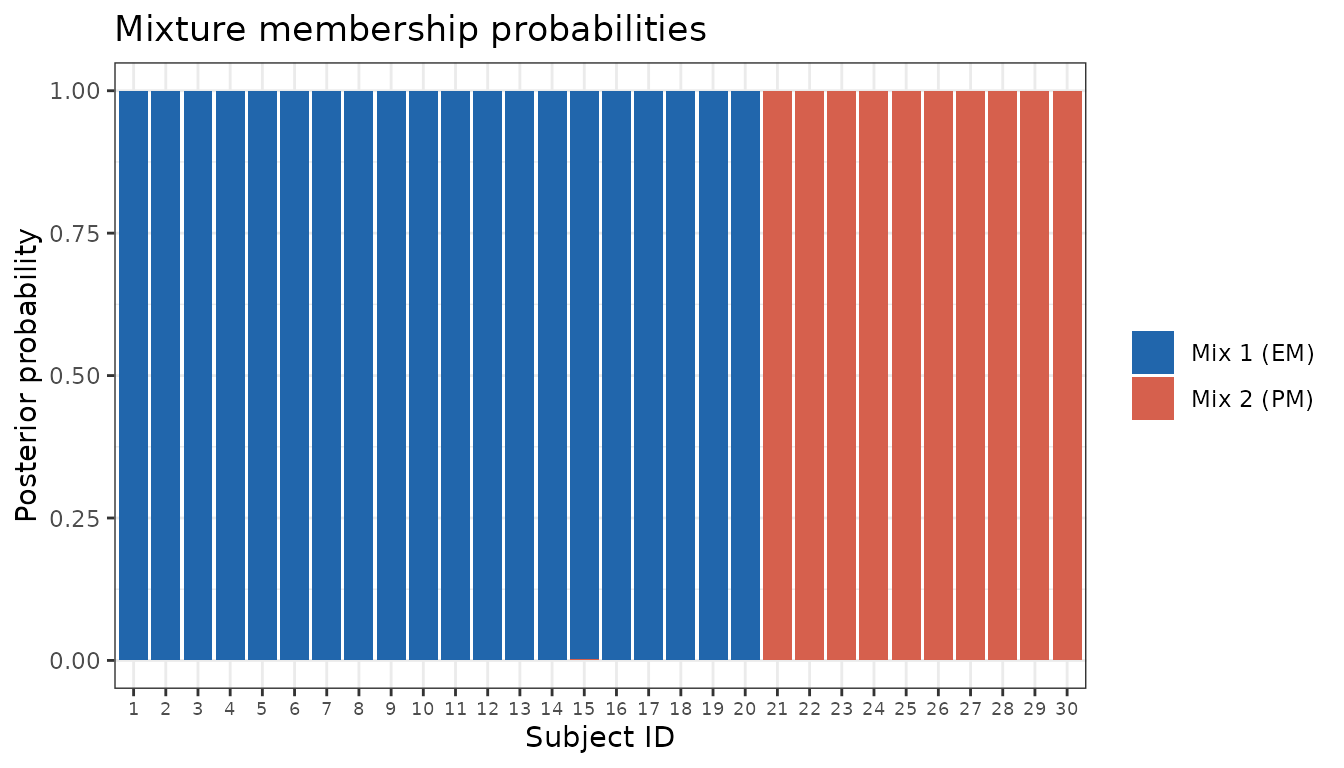

Most subjects will show a bar that is essentially 100% one colour, confirming clear separation of the two populations.

Mixture Models with SAEM

SAEM accepts the same mix() model syntax as the gradient-based methods, so the twoPop model defined above can be submitted to it directly:

fitSaem := nlmixr2(twoPop, simData, "saem",
                   control = saemControl(nBurn = 200, nEm = 300, print = 0))
print(fitSaem)
#> ── nlmixr² SAEM OBJF by FOCEi approximation ──
#> 
#>  Gaussian/Laplacian Likelihoods: AIC() or $objf etc. 
#>  FOCEi CWRES & Likelihoods: addCwres() 
#> 
#> ── Time (sec $time): ──
#> 
#>              setup   optimize covariance preprocess configure saem postprocess
#> elapsed 0.09751632 3.8433e-05  0.0350059      0.071     0.759 19.5       0.797
#>         table compress     other
#> elapsed 0.026    0.092 0.8464394
#> 
#> ── Population Parameters ($parFixed or $parFixedDf): ──
#> 
#>         Est.     SE  %RSE Back-transformed(95%CI) BSV(CV% or SD) Shrink(SD)%
#> tka    0.185 0.0347  18.8       1.20 (1.12, 1.29)                           
#> tcl1   -4.04                                 3.56                           
#> tcl2   -6.54                                0.389                           
#> tv      3.38 0.0330 0.977       29.5 (27.6, 31.4)           17.9       11.5 
#> p1     0.866 0.0980  11.3    0.866 (0.553, 0.971)                           
#> add.sd 0.326                                0.326                           
#> eta.cl                                                      1.10       29.2 
#>  
#>   Covariance Type ($covMethod): linFim
#>   Fixed parameter correlations in $cor
#>   No correlations in between subject variability (BSV) matrix
#>   Full BSV covariance ($omega) or correlation ($omegaR; diagonals=SDs) 
#>   Distribution stats (mean/skewness/kurtosis/p-value) available in $shrink 
#>   Information about run found ($runInfo):
#>    • error calculating tables, returning without table step 
#>    • diag(V) had non-positive or NA entries; the non-finite result may be dubious 
#>   Censoring ($censInformation): No censoring

tka and tv get real, finite SEs; tcl1/tcl2 (the mixture-owned fixed effects) correctly show no SE rather than either an error or a fabricated number — see the covariance callout below. p1 does now carry an SE: the proportion is reported at its score-zero point, which is the condition the mixture information matrix needs (see Standard errors for the mixture proportions).

Compare the back-transformed p1 above against the true EM prevalence of 0.67, and check that fitSaem$mixNum is a real rather than a collapsed split:

table(fitSaem$mixNum$mixnum)
#> 
#>  1  2 
#> 28  2

Cross-tabulated against the true labels. Which component gets index 1 is not fixed, so read the counts rather than the row labels (see the caution above):

compSaem <- merge(fitSaem$mixNum, truth, by = "ID")
compSaem$predicted <- ifelse(compSaem$mixnum == 1, "component 1", "component 2")
table(Predicted = compSaem$predicted, True = compSaem$trueGroup)
#>              True
#> Predicted     EM (fast) PM (slow)
#>   component 1        20         8
#>   component 2         0         2

SAEM typically separates these two subpopulations less cleanly than FOCEi does on the same data; the settings discussed next are what to reach for when it does.

Two known limitations, both distinct from component separation itself. First, tcl1/tcl2 (the mixture-owned fixed effects) show no SE. The linearized Fisher-information calculation degrades gracefully now — tka and tv get real SEs instead of the whole covariance matrix failing — but tcl1/tcl2 themselves remain genuinely under-identified from the linearization alone whenever few subjects are confidently assigned to the minority component, whether or not the components share an ETA (using split ETAs, see below, does not by itself fix this). Second, separation quality itself is sensitive to nBurn/nEm and to the mixProbPriorN/mixProbMethod settings described next — increasing mixProbPriorN to 30 and using nBurn = 400, nEm = 800 moves it toward FOCEi’s separation on this same simulated data. For a first look at a mixture model, or when precise per-subject classification matters, focei remains the more reliable default; SAEM is a usable alternative that may need more iterations and/or a higher mixProbPriorN to match it.

Why SAEM needs help separating mixture components

The gradient-based methods use a hard assignment: every subject is solved under each component, and the single best-fitting component is selected before the sufficient statistics are updated — this optimizes each subject independently on every iteration, so it cannot get stuck. SAEM instead uses a soft (probabilistic) assignment that fits naturally into its stochastic-approximation framework, but that same stochastic-approximation mechanism makes the mixing probability itself prone to a runaway positive-feedback collapse: the per-subject responsibility used to update it is weighted by the current mixing probability, so a small, noisy drift shrinks the responsibility of the shrinking component for every subject (not just the ones that truly belong to the other component), which shrinks the next iteration’s estimate further. Left unchecked this can drive the mixing probability all the way to exactly 0 or 1 well before the fixed effects have separated — saemControl()’s mixProbMethod (below) exists specifically to prevent that.

Stabilizing the mixing-probability estimate: `mixProbMethod`

saemControl() exposes three ways to stabilize the mixing probability against the collapse described above:

mixProbMethod = "regress" (the default). Skip the per-iteration soft-EM responsibility step altogether: each subject is hard-classified to a component once, up front, and that membership is held fixed and fed into the solve as a regressor. This avoids the feedback loop by construction and is the lowest-bias option. The cost is variance rather than bias — an early misclassification is never revisited — so prefer "regularized" when membership is genuinely uncertain. Because membership is fixed, the prob column of $mixList is 0/1 under this option rather than a graded posterior; use one of the other two if you want soft weights.
mixProbMethod = "regularized". Blend mixProbPriorN pseudo-subjects, distributed according to the model’s initial mixing probability (from ini()), into the responsibility average used at every iteration — equivalent to a Dirichlet-prior/MAP-EM correction on the mixing proportions. This changes what the estimate converges toward (pulled toward the initial guess, with the pull’s relative strength shrinking as the number of subjects grows), in exchange for reliably preventing collapse. Larger mixProbPriorN and more nBurn/nEm iterations both improve separation quality, as shown above.
mixProbMethod = "annealed". Give the mixing-probability update its own step-size schedule that decays from iteration 1 (mixProbStepExp), instead of the shared burn-in step of 1 used for ordinary parameters. This only slows how fast the estimate can move, without biasing what it converges to — but for a systematic (rather than purely noise-driven) collapse, slowing the walk to the same wrong answer does not, by itself, prevent reaching it. Prefer this when you want to avoid any bias toward the initial mixing probability and believe the components are already reasonably separated.

# more separation power, at the cost of more iterations and some bias
# toward the ini()-specified p1:
saemControl(mixProbMethod = "regularized", mixProbPriorN = 30,
            nBurn = 400, nEm = 800)

How SAEM handles mixtures differently

The gradient-based methods use a hard assignment: every subject is solved under each component, and the single best-fitting component is selected before the sufficient statistics are updated. SAEM instead uses a soft (probabilistic) assignment that fits naturally into its stochastic-approximation framework:

Per-component MCMC. At each iteration the SAEM kernel runs the MCMC sampling of the random effects once per mixture component, producing a separate set of posterior phi samples for each component.
Posterior membership weights. For every subject $i$ and component $k$ a posterior weight $a_{ik}$ is computed from the joint negative log-likelihood (observation loss plus the prior penalty on the random effects), combined with the current mixing probability $\pi_k$ : $a_{ik} \;=\; \frac{\pi_k \, \exp(-L_{ik})}{\sum_{j} \pi_j \, \exp(-L_{ij})}$ where $L_{ik}$ is the average joint negative log-likelihood of subject $i$ under component $k$ across the MCMC samples. Using the joint loss (rather than the observation loss alone) is essential: the MCMC adapts each subject’s ETAs to fit the data well under every component, so the prior penalty (the Mahalanobis distance of each sample from the component mean) is what discriminates which component truly fits.
Weighted sufficient statistics. The fixed-effect, $\Omega$ , and residual sufficient statistics are accumulated as $a_{ik}$ -weighted averages over all components rather than from a single selected component.
Stochastic-approximation update of the mixing probability. The population mixing probability is updated each iteration toward the mean posterior weight: $\pi_k^{(\text{new})} \;=\; \pi_k \;+\; \gamma_{\text{iter}}\, \bigl(\bar a_{\cdot k} - \pi_k\bigr)$ with $\gamma_{\text{iter}}$ the usual SAEM step-size sequence.

Because the assignment is soft, SAEM does not discard information from the non-selected components, which can improve stability when subpopulations are not perfectly separated.

Accessing SAEM mixture results

The same accessors are available as for the gradient-based fits, and return values without error:

fitSaem$mixNum         # most-likely component per subject (1-indexed)
#>    ID mixnum
#> 1   1      1
#> 2   2      1
#> 3   3      1
#> 4   4      1
#> 5   5      1
#> 6   6      1
#> 7   7      1
#> 8   8      1
#> 9   9      1
#> 10 10      1
#> 11 11      1
#> 12 12      1
#> 13 13      1
#> 14 14      1
#> 15 15      1
#> 16 16      1
#> 17 17      1
#> 18 18      1
#> 19 19      1
#> 20 20      1
#> 21 21      1
#> 22 22      1
#> 23 23      1
#> 24 24      1
#> 25 25      1
#> 26 26      1
#> 27 27      1
#> 28 28      2
#> 29 29      1
#> 30 30      2
fitSaem$mixList$mix1   # ID, ETAs, and posterior probability for component 1
#>    ID      eta.cl        eta.v       prob
#> 1   1  1.22313024  0.080196617 0.99808799
#> 2   2  0.94823717 -0.029125689 0.97182608
#> 3   3  0.73760829 -0.078017122 0.99857425
#> 4   4  0.67236040  0.336548189 0.99465605
#> 5   5  1.18687884 -0.062127160 0.99956467
#> 6   6  1.31844247  0.006551186 0.99898488
#> 7   7  0.96860163  0.189370375 0.99970155
#> 8   8  0.57726448 -0.061615831 0.96172145
#> 9   9  0.52439231 -0.106154856 0.98599779
#> 10 10  0.42431629  0.166748233 0.98180066
#> 11 11  0.33278360 -0.143461726 0.99463891
#> 12 12  1.04611033  0.050776557 0.99201421
#> 13 13  0.89135665 -0.072302958 0.99870011
#> 14 14  1.16413492  0.253394466 0.99976852
#> 15 15 -0.05241701 -0.209805243 0.97728563
#> 16 16  0.85643405  0.041459362 0.99180972
#> 17 17  0.39013412 -0.068722833 0.97319176
#> 18 18  1.08135554  0.068859707 0.99518599
#> 19 19  0.36096024  0.164010957 0.98105905
#> 20 20  0.23936294  0.208534429 0.98644132
#> 21 21 -0.73505303 -0.040457548 0.85343161
#> 22 22 -0.73681984 -0.285648214 0.71069034
#> 23 23 -0.62624561 -0.228119918 0.84957869
#> 24 24 -0.73138083 -0.086681842 0.75885570
#> 25 25 -0.68602817 -0.146293059 0.79211056
#> 26 26 -0.76444436 -0.251516101 0.64872589
#> 27 27 -0.69530604  0.078701577 0.54112511
#> 28 28 -0.68321755  0.008082041 0.46849596
#> 29 29 -1.04304263  0.235012419 0.50036911
#> 30 30 -0.67808768  0.012818381 0.08831775
fitSaem$mixProbabilities  # final population mixing probabilities (sum to 1)
#> [1] 0.8664237 0.1335763

A mixest/mixnum output variable works the same way here as for the gradient-based methods — see Reading the component off the fit table. For SAEM the component reported there is the hard assignment $mixNum records, which for mixProbMethod = "regress" (the default) is also what the fit itself conditioned on.

For SAEM, the prob column in $mixList is the membership weight $a_{ik}$ the SAEM engine computed directly (returned internally as the mixWeights matrix), and $mixNum reports the component with the largest weight. Under the default mixProbMethod = "regress" that weight is 0/1, because membership was hard-classified once rather than updated as a responsibility — a valid MAP assignment, but not a graded posterior. Switch to "regularized" or "annealed" if you want to see how uncertain each subject’s membership is.

$etaExpected holds the posterior-weighted ETAs used for shrinkage. These are meaningful once mixProbMethod is keeping the fit stable, but their precision (how many subjects land in the correct component) depends on the number of iterations — and, under "regularized", on mixProbPriorN — more so than for the gradient-based methods.

Shared variability across components (split ETAs)

A component expression may use its own random effect — for example mix(expit(tcl1 + eta.cl1, ...), p1, expit(tcl2 + eta.cl2, ...)), where eta.cl1 and eta.cl2 are separate ETAs sharing the same root name. SAEM detects these split ETAs and collapses them back to a single between-subject variability term in the reported $omega. The shared variance is computed with the law of total variance using the posterior weights as component sizes: $\operatorname{Var}(\eta) \;=\; \underbrace{\sum_k w_k\,\sigma_k^2}_{\text{mean of variances}} \;+\; \underbrace{\sum_k w_k\,(\mu_k - \bar\mu)^2}_{\text{variance of means}}, \qquad w_k = \frac{\sum_i a_{ik}}{\sum_i \sum_j a_{ij}}$ so a single eta.cl term is reported even though each component was sampled with its own random effect during estimation.

twoPopSplit <- function() {
  ini({
    tka   <- log(1.2)
    tcl1  <- logit(0.8, 0.1, 200)
    tcl2  <- logit(0.8, 0.1, 200)
    tv    <- log(30)
    p1    <- 0.67
    eta.cl1 ~ 0.09
    eta.cl2 ~ 0.09
    eta.v  ~ 0.04
    add.sd <- 0.2
  })
  model({
    ka <- exp(tka)
    cl <- mix(expit(tcl1 + eta.cl1, 0.1, 200), p1, expit(tcl2 + eta.cl2, 0.1, 200))
    v  <- exp(tv + eta.v)
    linCmt() ~ add(add.sd)
  })
}
fitSaemSplit := nlmixr2(twoPopSplit, simData, "saem",
                        control = saemControl(nBurn = 200, nEm = 300, print = 0,
                                              covMethod = "linFim"))
print(fitSaemSplit)
#> ── nlmixr² SAEM OBJF by FOCEi approximation ──
#> 
#>  Gaussian/Laplacian Likelihoods: AIC() or $objf etc. 
#>  FOCEi CWRES & Likelihoods: addCwres() 
#> 
#> ── Time (sec $time): ──
#> 
#>              setup   optimize covariance preprocess configure  saem postprocess
#> elapsed 0.06767546 3.2336e-05 0.08400512      0.065     1.114 8.523       0.514
#>         table compress    other
#> elapsed 0.016    0.209 1.032287
#> 
#> ── Population Parameters ($parFixed or $parFixedDf): ──
#> 
#>         Est.     SE %RSE Back-transformed(95%CI) BSV(CV% or SD) Shrink(SD)%
#> tka    0.321 0.0492 15.3       1.38 (1.25, 1.52)                           
#> tcl1   -3.50                                5.94                           
#> tcl2   -5.83                               0.684                           
#> tv      3.47 0.0357 1.03       32.1 (29.9, 34.4)           19.1        100 
#> p1     0.667 0.0861 12.9    0.667 (0.484, 0.810)                           
#> add.sd 0.414                               0.414                           
#> eta.cl                                                     1.10       85.0 
#>  
#>   Covariance Type ($covMethod): linFim
#>   Fixed parameter correlations in $cor
#>   No correlations in between subject variability (BSV) matrix
#>   Full BSV covariance ($omega) or correlation ($omegaR; diagonals=SDs) 
#>   Distribution stats (mean/skewness/kurtosis/p-value) available in $shrink 
#>   Information about run found ($runInfo):
#>    • error calculating tables, returning without table step 
#>    • diag(V) had non-positive or NA entries; the non-finite result may be dubious 
#>   Censoring ($censInformation): No censoring

Split ETAs correctly separate the two clearances (5.98 and 0.71, near the true 8 and 0.8) instead of collapsing together — as with the non-split example above, tcl1/tcl2 still show no SE from the linearization, and this particular run’s reported eta.cl BSV (1.08 SD) is not trustworthy (true value: 0.3 SD) — see the callout below.

Prefer a truly mu-referenced parameterization when you can

tcl1 + eta.cl1 above is nested inside expit(...), so cl itself is a nonlinear function of the mu-referenced quantity. If your parameter doesn’t need a hard bound, write the mixture directly in terms of the mu-referenced value with no wrapper, e.g. cl <- mix(tcl1 + eta.cl1, p1, tcl2 + eta.cl2) with tcl1/tcl2 initialized directly to a clearance guess (not a log/logit-scale one). On the same simulated data this recovers 7.5–7.6 and 0.64–0.67 across seeds — closer to the true 8/0.8 than the bounded form above — because SAEM’s per-component weighted update (used to keep tcl1/tcl2 from being diluted by each other, described next) is an exact weighted-least-squares fit when the mu-referenced quantity has no nonlinear wrapper, and a wrapped/bounded parameterization tends to compress the two components closer together in the space the likelihood actually sees, weakening separation. Prefer the bounded form only when you genuinely need a hard constraint (e.g. a rate that must stay positive) that the data can’t be trusted to respect on its own.

No parameterization prevents label switching. Whichever form you use, there is no way to pin down which mixture component ends up as component 1 vs. component 2 without adding a boundary/ordering constraint to the parameter — and adding one (e.g. wrapping in logit()/bounding tcl1 below tcl2) requires a nonlinear transform, which is exactly the “wrapped” form the previous paragraph recommends against for separation quality. So the order of tcl1/tcl2 (which one comes out larger) — and correspondingly which numeric label mixNum assigns to which true subpopulation — can differ from run to run or across seeds. Always check the estimated values (or cross-tabulate mixNum against known labels, as in the classification example above) rather than assuming tcl1 is always “the fast/EM group.”

The BSV/$omega issue above is independent of parameterization. Whether you use the bounded or the mu-referenced form, split ETAs’ reported variability can still come out wrong (too large or collapsed near zero) even when the fixed effects themselves separate correctly. Treat $omega/BSV% for split-ETA mixture components as unreliable for now; the point estimates of tcl1/tcl2 and p1 are the numbers to trust.

An alternative sampling architecture: `mixSampleMethod = "msaem"`

The BSV problem above comes from how SAEM’s default architecture explores the random effects for a mixture. saemControl(mixSampleMethod=) selects between two designs:

"parallel" (default). Every iteration, one full MCMC chain is run per component for every subject (each chain explores as if that subject definitely belongs to that component), then the results are blended post hoc using posterior weights. This mirrors NONMEM’s population mixture modeling ($MIX) and correctly estimates a single BSV shared across all components — but it has no way to obtain a clean per-component BSV for split-ETA models: each “wrong-hypothesis” chain still explores its non-owned column(s) as an unconstrained prior-only random walk, and that noise ends up in the blended statistics.
"msaem" (experimental). Implements MSAEM (Lavielle & Mbogning 2014, Statistics and Computing 24(5)), the method Monolix uses for mixture models: only one random-effects trajectory is simulated per subject per iteration, and the discrete component label is analytically marginalized out via an exact posterior responsibility instead of being simulated — so there is nothing to blend after the fact. It also uses a model-aware stratified initialization (each subject is tested against every candidate component using the actual compiled model before fitting starts), which reliably separates split-ETA fixed effects even from the realistic symmetric starting point used throughout this vignette (tcl1/tcl2 both initialized identically).

"parallel" runs nMix full chains per subject per iteration where "msaem" runs one, so they are not compute-matched at equal nmc — set nmc to roughly nMix times its default (nmc = 6 for a 2-component mixture here) for a fair comparison:

fitSaemMsaem := nlmixr2(twoPopSplit, simData, "saem",
                        control = saemControl(nBurn = 200, nEm = 300, nmc = 6,
                                              print = 0,
                                              mixSampleMethod = "msaem",
                                              covMethod = "linFim"))
print(fitSaemMsaem)
#> ── nlmixr² SAEM OBJF by FOCEi approximation ──
#> 
#>  Gaussian/Laplacian Likelihoods: AIC() or $objf etc. 
#>  FOCEi CWRES & Likelihoods: addCwres() 
#> 
#> ── Time (sec $time): ──
#> 
#>              setup   optimize covariance preprocess configure  saem postprocess
#> elapsed 0.06265187 3.1495e-05 0.01300518      0.051     0.142 16.71       0.318
#>         table compress     other
#> elapsed 0.016    0.129 0.2213115
#> 
#> ── Population Parameters ($parFixed or $parFixedDf): ──
#> 
#>         Est.     SE  %RSE Back-transformed(95%CI) BSV(CV% or SD) Shrink(SD)%
#> tka    0.124 0.0403  32.4       1.13 (1.05, 1.23)                           
#> tcl1   -5.45                                0.954                           
#> tcl2   -3.38                                 6.70                           
#> tv      3.36 0.0333 0.990       28.8 (27.0, 30.8)           17.9       49.5 
#> p1     0.333 0.0861  25.8    0.333 (0.190, 0.516)                           
#> add.sd 0.391                                0.391                           
#> eta.cl                                                     0.987       84.7 
#>  
#>   Covariance Type ($covMethod): linFim
#>   Fixed parameter correlations in $cor
#>   No correlations in between subject variability (BSV) matrix
#>   Full BSV covariance ($omega) or correlation ($omegaR; diagonals=SDs) 
#>   Distribution stats (mean/skewness/kurtosis/p-value) available in $shrink 
#>   Information about run found ($runInfo):
#>    • error calculating tables, returning without table step 
#>    • diag(V) had non-positive or NA entries; the non-finite result may be dubious 
#>   Censoring ($censInformation): No censoring

Fixed effects separate about as well as "parallel" — tcl1 and tcl2 back-transform to 0.954 and 6.7 against the true 0.8 and 8. The usual label-order caveat applies: which component gets index 1 is not fixed, so compare the two back-transformed clearances against what you expect each subpopulation to be before reading anything else in the row.

The raw, unpooled per-component BSV (fitSaemMsaem$env$saem0$Gamma2_phi1) is better than "parallel"’s, whose equivalent raw diagonal is always exactly zero for split-ETA columns (the pooled $omega shown in parFixed only looks reasonable because pooling adds in the between-component variance of the means) — but it is still not a reliable recovery of the true 0.09.

And read p1 against the component it actually belongs to. p1 is the prior probability of component 1, which in this fit is the component whose clearance is 0.954 — so compare it to that subpopulation’s true fraction, not automatically to the 0.67 the earlier examples use. That mismatch, not a fitting failure, is what makes a swapped run look wrong at first glance.

Bottom line: "msaem"’s fixed-effect separation is as solid as "parallel"’s, and its split-ETA BSV, while still not reliable, is closer to the truth than "parallel"’s (which is always exactly zero underneath the pooled report). It remains experimental — mixProb can be less accurate, and BSV recovery is inconsistent across datasets/seeds. Prefer "parallel" (the default) unless you are specifically evaluating "msaem" or comparing the two.

Other estimation families

Mixture support is not limited to the gradient-based methods and SAEM. Two more families accept mix() and return the same $mixNum/$mixList accessors and the same mixest/mixnum table columns.

The EM / importance-sampling family: `imp`, `impmap`, `qrpem`

These are part of the same FOCEi family as the gradient-based methods and reach the mixture the same way — ETAs are optimized for every subject x component combination and the best-fitting component is selected, exactly as described in Accessing Mixture Results — so $mixNum and $mixList$prob mean the same thing here as they do for focei. What differs is how the individual marginal likelihood is obtained: by importance sampling rather than by a Laplace-style linearization.

fitImp := nlmixr2(twoPop, simData, "imp", control = impControl(print = 0))
fitImp$parFixed
#>         Est.     SE %RSE Back-transformed(95%CI) BSV(CV% or SD) Shrink(SD)%
#> tka    0.170 0.0530 31.2       1.18 (1.07, 1.31)                           
#> tcl1   -4.69  0.228 4.86       1.91 (1.26, 2.92)                           
#> tcl2   -4.47  0.361 8.09       2.37 (1.23, 4.66)                           
#> tv      3.38 0.0491 1.45       29.4 (26.7, 32.4)           18.6       13.2<
#> p1     0.762    NaN  NaN        0.762 (NaN, NaN)                           
#> add.sd 0.328 0.0141 4.29    0.328 (0.300, 0.355)                           
#> eta.cl                                                     1.31       9.27<

They are a reasonable middle ground: no linearization error, and, because the component assignment is the family’s hard assignment rather than a soft-EM responsibility, no mixing-probability collapse to guard against — at the cost of the Monte-Carlo sampling itself. impmap re-centres the sampling on the MAP estimate and qrpem uses a quasi-random sequence, both of which reduce the sampling variance relative to plain imp at the same number of draws.

The nonparametric family: `npag`, `npb`

A nonparametric distribution is already a mixture

This needs stating plainly, because it is easy to reach for mix() here out of habit and get nothing for it.

npag (adaptive grid) and npb (Dirichlet-process Bayesian) do not assume the random effects are normal. They estimate a discrete distribution — a set of support points $\phi_k$ with weights $w_k$ — and the marginal likelihood of a subject is

$p(y_i) \;=\; \sum_k w_k \, p(y_i \mid \phi_k)$

which is a mixture already, over the support points, with as many components as the data will support and each subject carrying a posterior over them. Two distinct subpopulations do not need to be declared: the grid puts mass in two places, and the two groups of subjects separate on their own. If all you mean is “clearance is bimodal”, a nonparametric fit gives you that without mix(), without committing to how many modes there are, and without needing initial estimates for each one.

So what does `mix()` add?

The two describe different things, and they sit at different levels of the model:

	What varies	How many	Estimated as
Nonparametric support	the random effects — where subjects sit in the parameter space	discovered from the data	support points and weights
`mix()`	the structural model — a different fixed-effect expression per subpopulation	declared by you	per-component thetas plus a proportion

A support point is an unlabeled location in the random-effect space. A mix() component is a claim that some subjects follow a different equation: a different typical clearance parameter, a different absorption model, a different anything you can write on the right-hand side. That is not something a support distribution can express, because every support point is evaluated through the same structural model.

So declare mix() on top of a nonparametric method when you want the things only a declared mixture gives you — a named, estimated proportion you can report and test, a per-component fixed effect with its own interpretation, a per-subject component assignment tied to a mechanism (a genotype, a formulation, a disease state) — and let the nonparametric distribution keep doing what it is for, describing the spread within each of those components without assuming it is normal. Reach for the nonparametric fit alone when the multimodality is the finding rather than the hypothesis.

How the two are fitted together

One nonparametric distribution is shared across the declared components — the support set is not re-estimated per component. Each subject is split into per-component pseudo-subjects and the conditional likelihood is marginalized over the components using the mixing proportions, $p(y_i \mid \phi) = \sum_m \pi_m\, p(y_i \mid \phi, m)$ . npag then updates the proportion once per cycle with an EM step, holding the support points and weights fixed; npb samples it inside its blocked Gibbs sweep — each subject draws a component from its posterior responsibility and the proportions are drawn from $\mathrm{Dirichlet}(1 + \text{component counts})$ , with the posterior-mean proportions reported in $env$npbMixProb. A fix()ed proportion is held at its ini() value in both.

The components’ own structural parameters (the per-component typical clearance, say) are estimated alongside the residual parameters against that same marginalized conditional likelihood — they are estimated, not held at their initial values. Only the proportions are handled by the separate update step above.

fitNpag := nlmixr2(twoPop, simData, "npag", control = npagControl(print = 0))
fitNpag$parFixed
#>         Est.     SE %RSE Back-transformed(95%CI) BSV(CV% or SD) Shrink(SD)%
#> tka    0.192 0.0527 27.4       1.21 (1.09, 1.34)                           
#> tcl1   -4.29  0.430 10.0       2.81 (1.28, 6.29)                           
#> tcl2   -4.88   1.10 22.6      1.61 (0.274, 12.5)                           
#> tv      3.40 0.0467 1.37       30.0 (27.4, 32.8)           20.0       14.9<
#> p1     0.604  0.961  159   0.604 (5.80e-4, 1.00)                           
#> add.sd 0.316 0.0139 4.39    0.316 (0.289, 0.343)                           
#> eta.cl                                                     1.09      -2.17>

Methods that decline a mixture

emvi and fbvi (mean-field variational inference) stop up front with

'twoPop' cannot have a mixture model (ie `mix()`) for the estimation routine 'emvi'

rather than silently fitting a model without the mixture structure.

vae does fit a mixture model. It follows the same convention as the gradient-based methods – every subject-component pair is characterized by the encoder at its own eta, membership is the posterior responsibility, and the proportions are estimated on the mlogit scale through their analytic gradient – so a mix() model can be submitted to it directly. Earlier versions stopped during assembly rather than fitting.

Choosing an Estimation Method

All six gradient-based methods handle mixture models using the same strategy: ETAs are optimized separately for every subject × mixture combination and the best-fitting component is selected. This works reliably in practice and gives the cleanest separation. SAEM’s scheme is described in Mixture Models with SAEM; its default, mixProbMethod = "regress", hard-classifies rather than collapsing, but it may still separate components less precisely than the gradient-based methods on small/weakly-separated datasets. Where membership is genuinely uncertain, switch to mixProbMethod = "regularized" and raise mixProbPriorN and nBurn/nEm (mixProbPriorN applies only to "regularized"; see that section for a worked example):

Method	Interaction	Accuracy	Notes
`focei`	Yes	High	Recommended; full FOCE with interaction
`foce`	No	High	Like FOCEI without η–ε interaction
`laplace`	Yes	High	Good alternative to FOCEI
`agq`	Yes	Highest	Most accurate; slowest
`fo`	No	Low	Linearization; fast but less accurate
`foi`	Yes	Low	FO with interaction
`saem`	Yes	Moderate–High	Hard-classifies by default (`mixProbMethod = "regress"`); for uncertain membership use `"regularized"` and tune `mixProbPriorN`/`nBurn`/`nEm`; see Mixture Models with SAEM
`imp` / `impmap` / `qrpem`	Yes	High	Same hard assignment as FOCEi, marginal likelihood by importance sampling; see Other estimation families
`npag` / `npb`	Yes	—	Nonparametric random effects; marginalizes over components. Consider whether you need `mix()` at all — see Other estimation families

Notes and Limitations

Computational cost is multiplied by the number of mixture components, because the inner optimization runs for nSub × nMix individuals (or, for SAEM, nMix MCMC passes per iteration).
Identifiability requires that the mixture components are well-separated in the data. More than 2–3 components is rarely supportable with typical PK/PD datasets.
A proportion sitting at 0 or 1 is the usual sign that a component is not supported by the data. Its reported SE will be very small, which is the correct delta-method answer and not evidence of precision — see Standard errors for the mixture proportions.
The mixest, mixnum, and mixunif variables can be included in the model block for diagnostic purposes but do not affect the likelihood. mixest and mixnum report the fitted component and the component count in the fit table (see Reading the component off the fit table); mixunif is only meaningful when simulating.
Initial estimates matter: provide lower bounds on tcl1 and tcl2 to prevent label-switching for focei during optimization. They matter at least as much for SAEM under its default mixProbMethod = "regress", which hard-classifies every subject once, up front, and never revisits that assignment — so a poor start is not corrected by later iterations. Where membership is genuinely uncertain, prefer "regularized".
SAEM supports mixtures via an EM-responsibility (soft assignment) scheme whose default, mixProbMethod = "regress", hard-classifies each subject once rather than updating responsibilities, and correctly separates split-ETA fixed effects under both mixSampleMethod options (see Mixture Models with SAEM); it typically needs more tuning than the gradient-based methods to match their separation precision — more nBurn/nEm, and, if you switch to "regularized" for uncertain membership, a larger mixProbPriorN (which applies to that option only). Two things it does not currently do well regardless of parameterization or mixSampleMethod: standard errors for the mixture-owned fixed effects (tcl1/tcl2-style parameters) come back as NA rather than a real SE (the mixture proportion does get one under the gradient-based methods — see Standard errors for the mixture proportions), and $omega/BSV for split-ETA components can be unreliable (too large or collapsed near zero under mixSampleMethod="parallel", the default; improved but still not consistently accurate under the experimental "msaem") even when the fixed effects themselves separate correctly — trust the point estimates of tcl1/tcl2/p1, not their SEs or BSV%. Nested transforms inside mix() require rxode2 >= 5.1.3 regardless of estimation method.