Importance-sampling EM in nlmixr2: imp, impmap and qrpem

nlmixr

The importance-sampling EM family

nlmixr2 provides three closely related Monte-Carlo expectation-maximization estimators, all built on one importance-sampling kernel and differing only in how the per-subject E-step is sampled:

est = "imp" – importance sampling with the proposal centered at each subject’s running conditional mean. This is similar to NONMEM’s METHOD=IMP.
est = "impmap" – importance sampling with the proposal centered at each subject’s MAP mode, using the inner (conditional) Hessian as covariance. This is similar to NONMEM’s METHOD=IMPMAP.
est = "qrpem" – the same EM but with Sobol quasi-random importance samples and a SIR-accelerated M-step. This is similar to the quasi-random parametric EM of Leary & Dunlavey (2012) – the method Phoenix NLME made its flagship. qrpemControl() is exactly impmapControl(qr = TRUE, sir = TRUE).

What unites them, and separates them from FOCEI, is that they evaluate the marginal likelihood by Monte-Carlo integration rather than by a Laplace approximation. Each one draws samples for every subject from a proposal distribution aimed at that subject’s posterior, then re-weights those samples to undo the aiming. The three differ only in how the proposal is aimed and how the samples are drawn.

This article is ordered practically: when to reach for these methods, a worked example, and the parameters worth knowing come first. How it works explains the algorithm in plain terms afterwards, and Appendix A walks step by step through NONMEM’s IMP/IMPMAP, marking what is the same and what is different.

When to use these methods

Reach for imp / impmap / qrpem when:

you need a trustworthy marginal likelihood and do not trust FOCEI’s Laplace approximation – strongly nonlinear models, sparse data, or non-normal (categorical, count, ordered-categorical, time-to-event) endpoints, where the posterior is genuinely non-Gaussian. These fits report the Laplace and the Monte-Carlo likelihood side by side, so the gap between them tells you how much the approximation was costing you (see below);
you want a fit that is methodologically comparable to NONMEM IMP/IMPMAP or to Phoenix QRPEM, e.g. to cross-check a submission run;
you want importance-sampling standard errors (covMethod = "imp", the default) computed from the same Monte-Carlo likelihood rather than a Laplace or sandwich estimator;
FOCEI is struggling to converge but you still want a likelihood-based fit; the EM update is monotone in expectation and does not depend on an outer quasi-Newton search.

Which of the three (the proposals are compared in detail further down):

impmap is the sensible default of the family. The MAP-centered proposal is the best-aimed one, so it needs the fewest samples – as long as the mode search behaves.
imp when the per-iteration MAP search is unstable or expensive: flat or multimodal individual posteriors, or a model where the inner problem is slow. It is cheaper per iteration and more forgiving, at the cost of needing more samples.
qrpem when Monte-Carlo noise is your binding constraint – you want a reproducible objective, or you want to cut isample hard on an expensive model.

Stay with FOCEI when the model is close to linear and you want the fastest deterministic fit. Use SAEM when the likelihood is difficult or multimodal and a robust MCMC E-step is worth the cost – SAEM and the imp family are complementary, both EM, differing in how the E-step is done.

Two current limits to know: the imp family leans into mu-referencing (muModel = "lin"; this is what makes the M-step cheap), but allows non mu-referenced parameters at a cost.

Worked example

We use the theophylline data (theo_sd) and a one-compartment oral model with between-subject variability on ka, cl and v.

library(nlmixr2)

impModel <- function() {
  ini({
    tka <- 0.45
    tcl <- 1
    tv <- 3.45
    eta.ka ~ 0.6
    eta.cl ~ 0.3
    eta.v ~ 0.1
    add.sd <- 0.7
  })
  model({
    ka <- exp(tka + eta.ka)
    cl <- exp(tcl + eta.cl)
    v  <- exp(tv  + eta.v)
    d/dt(depot)  <- -ka * depot
    d/dt(center) <-  ka * depot - cl / v * center
    cp <- center / v
    cp ~ add(add.sd)
  })
}

Only est = changes across all five methods:

fitFocei  := nlmixr2(impModel, nlmixr2data::theo_sd, est = "focei",
                     control = foceiControl(print = 0L))
fitSaem   := nlmixr2(impModel, nlmixr2data::theo_sd, est = "saem",
                     control = saemControl(nBurn = 200L, nEm = 300L, print = 0L))
fitImp    := nlmixr2(impModel, nlmixr2data::theo_sd, est = "imp",
                     control = impControl(print = 0L))
fitImpmap := nlmixr2(impModel, nlmixr2data::theo_sd, est = "impmap",
                     control = impmapControl(print = 0L))
fitQrpem  := nlmixr2(impModel, nlmixr2data::theo_sd, est = "qrpem",
                     control = qrpemControl(print = 0L))

round(rbind(FOCEI  = fitFocei$theta,  SAEM   = fitSaem$theta,
            imp    = fitImp$theta,    impmap = fitImpmap$theta,
            qrpem  = fitQrpem$theta), 3)
#>          tka   tcl    tv add.sd
#> FOCEI  0.465 1.012 3.460  0.695
#> SAEM   0.452 1.014 3.451  0.698
#> imp    0.461 1.008 3.454  0.697
#> impmap 0.461 1.007 3.454  0.697
#> qrpem  0.458 1.012 3.454  0.698

All five recover the same parameters – theophylline is close to linear, so there is nothing here for a Monte-Carlo likelihood to rescue. The interesting part is the pair of objective functions each imp fit carries.

Two objectives: which number is which

This trips people up, so it is worth being explicit. An imp/impmap/qrpem fit reports two different -2LL values:

fit$objf – the value printed by print(fit) and used by AIC()/BIC() – is the FOCEI (Laplace) objective evaluated at the converged EM estimates. It is labelled FOCEi in fit$objDf. This is what makes it directly comparable to a focei fit of the same model.
fit$env$impObj is the importance-sampling -2LL: the Monte-Carlo evaluation of the marginal likelihood, from the final E-step.

Why the same machinery gives two different numbers

The obvious objection is that impmap is built on FOCEI, so how can it disagree with FOCEI? The answer is that they share the integrand, not the integration.

What impmap borrows from focei is the entire inner problem: the per-subject conditional-mode search, the inner Hessian at that mode, and the routine that evaluates the joint density p(y_i | eta) p(eta) at an arbitrary eta. These are literally the same functions est = "focei" calls – which is why impmap inherits FOCEI’s inner tolerances, its handling of censored (M2/M3/M4) data, and its mu-referencing machinery.

What the two do with that machinery is where they part company:

	uses mode + Hessian to…	so the objective is
FOCEI	substitute into the closed-form Gaussian integral	the Laplace approximation of `-2LL`
imp family	aim a proposal to draw samples from	a Monte-Carlo estimate of the same `-2LL`

FOCEI treats the mode and Hessian as the answer – it assumes the integrand is Gaussian and uses that Gaussian’s known area. The imp family treats them only as a good guess at where the mass is, draws from that guess, and then lets the importance weights correct for however wrong the guess was.

Two consequences worth being clear about:

They are on the same scale. Both carry the same normalizing constants (the -0.5 log|Omega| prior term and the rest), so both are estimates of the same quantity, in the same units. The difference between them is not an offset or a convention – it is the error the Laplace step is making.
They are evaluated at the same parameters. After the EM converges, nlmixr2 runs one final FOCEI MAP pass at the converged estimates to produce fit$objf. So the two numbers differ only in how the integral was done – same model, same data, same theta, same Omega, same modes. That is what makes their gap interpretable as the approximation error rather than as two methods disagreeing about where the optimum is.

impObjTable <- function(fit, label) {
  data.frame(method = label,
             `FOCEi -2LL (fit$objf)` = round(fit$objf, 3),
             `IS -2LL (impObj)`      = round(fit$env$impObj, 3),
             check.names = FALSE)
}
rbind(impObjTable(fitImp,    "imp"),
      impObjTable(fitImpmap, "impmap"),
      impObjTable(fitQrpem,  "qrpem"),
      data.frame(method = "focei", `FOCEi -2LL (fit$objf)` = round(fitFocei$objf, 3),
                 `IS -2LL (impObj)` = NA_real_, check.names = FALSE))
#>   method FOCEi -2LL (fit$objf) IS -2LL (impObj)
#> 1    imp               116.832          118.133
#> 2 impmap               116.838          118.035
#> 3  qrpem               116.831          118.106
#> 4  focei               116.804               NA

The gap between the two columns is the error in the Laplace approximation for this model – a diagnostic you cannot get from a FOCEI fit alone. Even on near-linear theophylline it is worth about 1.2 -2LL units, and the sign is informative: Laplace is optimistic here. The gap grows with the nonlinearity of the model, with sparse data, and with non-normal (categorical, count, ordered-categorical, time-to-event) endpoints – and in those cases the importance-sampling column is the trustworthy one.

Compare like with like: fit$objf against another fit$objf, or impObj against another impObj. Not because the two are in different units – as above, they are estimates of the same quantity on the same scale – but because mixing them mixes two estimators. Across a pair of nested models the Laplace error is often similar in both fits and largely cancels in the difference, so a objf-vs-objf comparison can be sound even when each number is individually biased; pit one against an impObj and you are reading that bias as if it were signal. Within a single fit, the gap between them is exactly the diagnostic described above.

(SAEM’s objective uses a separate likelihood evaluation and a different constant again, so compare SAEM to SAEM.)

Watching the EM run

Every imp-family fit stashes its per-iteration diagnostics on the fit environment. These are the first thing to look at when a fit misbehaves:

impDiag <- function(fit, label) {
  e <- fit$env
  data.frame(method       = label,
             iterations   = e$impIter,
             converged    = e$impConverged,
             `IS -2LL`    = round(e$impObj, 3),
             `ESS frac`   = round(tail(e$impNeffFrac, 1), 3),
             gamma        = e$impGammaUsed,
             isample      = e$impNsample,
             check.names  = FALSE)
}
rbind(impDiag(fitImp, "imp"), impDiag(fitImpmap, "impmap"),
      impDiag(fitQrpem, "qrpem"))
#>   method iterations converged IS -2LL ESS frac gamma isample
#> 1    imp        100     FALSE 118.133    0.922  1.25     300
#> 2 impmap        100     FALSE 118.035    0.962  1.00     300
#> 3  qrpem        100     FALSE 118.106    0.965  1.00     300

The two that matter most:

ESS frac (fit$env$impNeffFrac) is the effective sample size as a fraction of isample – how many of your samples are actually doing work. If it collapses toward 0, the proposal is missing the posterior and the estimates are being driven by a handful of samples.

Do not read a high value as better. Under the default gammaRule = "target" the sampler deliberately widens the proposal until xi reaches iaccept, which lowers this fraction on purpose – around 0.7 on theophylline against 0.96 under "floor" – in exchange for weights whose variance is bounded. A fraction near 1.0 means the proposal is narrow and matches the posterior closely, which is good only if its tails also do; impPsisK is what tells you that, and it is exactly the case where this statistic cannot (see below).
converged (fit$env$impConverged) is TRUE only if all three gates are met simultaneously in a trailing window: the objective has stopped moving, the parameters have stopped drifting, and gamma has settled. FALSE means the fit ran out its nIter budget – which, as below, is common at the default settings and is not automatically a problem. Look at the trace before reacting.

library(ggplot2)

traceOf <- function(fit, label) {
  e <- fit$env
  rbind(data.frame(method = label, iter = seq_along(e$impObjTrace),
                   what = "importance-sampling -2LL", value = e$impObjTrace),
        data.frame(method = label, iter = seq_along(e$impNeffFrac),
                   what = "effective sample fraction", value = e$impNeffFrac))
}
traces <- rbind(traceOf(fitImp, "imp"), traceOf(fitImpmap, "impmap"),
                traceOf(fitQrpem, "qrpem"))

ggplot(traces, aes(iter, value, colour = method)) +
  geom_line() +
  facet_wrap(~ what, scales = "free_y", ncol = 1) +
  labs(x = "EM iteration", y = NULL, colour = NULL,
       title = "The E-step settles quickly; the residual wobble is Monte-Carlo noise") +
  theme_bw()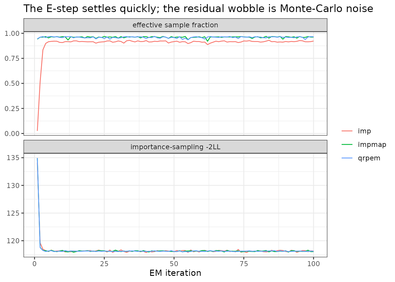

Two features of that plot are worth naming.

The effective sample fraction starts near zero and climbs. On iteration 1 the starting parameters are poor, so a proposal aimed with them lands badly and almost every sample is wasted; as the fit improves, the proposal starts matching the posterior and the fraction climbs. A fit whose ESS fraction never climbs is a fit whose proposal is wrong.

Under the default "target" rule it climbs and then settles below its peak, because the proposal-scale controller widens the proposal until xi reaches iaccept. That plateau is the controller working, not the fit degrading. Under gammaRule = "floor" it simply climbs and stays.

The objective flattens fast and then wobbles. That wobble is Monte-Carlo noise, not a failure to converge, and its size is set by isample. The default convergence test asks that the average absolute objective change over a 10-iteration window be under ctol (10^-sigdig, so 1e-4 relative by default). At isample = 300 the per-iteration noise on this model is roughly 0.1 in the -2LL, which is an order of magnitude larger than that gate, so the fit runs its full nIter budget and reports converged = FALSE while sitting on a perfectly good answer. If you want the flag to mean something, either raise isample (less noise) or relax ctol – see the parameters section below.

Why quasi-random (QRPEM): less Monte-Carlo noise for the same cost

That wobble is precisely the problem QRPEM attacks. Pseudo-random samples fill the parameter space unevenly – clumps here, gaps there – so the integration error shrinks only as 1 / sqrt(N). Sobol low-discrepancy (quasi-random) points fill it evenly by construction, shrinking the error much faster. The payoff: for the same (small) number of importance samples, qrpem gives a far more reproducible objective than pseudo-random imp.

Fit both at a deliberately small isample = 30 across several seeds and compare the spread of the converged objective:

seedStudy := local({
  seeds <- 1:5
  do.call(rbind, lapply(c("imp", "qrpem"), function(m) {
    objf <- vapply(seeds, function(s) {
      ctl <- if (m == "imp")
        impControl(print = 0L, isample = 30L, nIter = 80L, impSeed = s)
      else
        qrpemControl(print = 0L, isample = 30L, nIter = 80L, impSeed = s)
      suppressWarnings(as.numeric(nlmixr2(impModel, nlmixr2data::theo_sd,
                                          est = m, control = ctl)$objf))
    }, numeric(1))
    data.frame(method = m, seed = seeds, objf = objf)
  }))
})

## seed-to-seed spread of the converged -2LL
aggregate(objf ~ method, seedStudy, function(x) c(sd = sd(x), range = diff(range(x))))
#>   method     objf.sd  objf.range
#> 1    imp 0.246108416 0.598726708
#> 2  qrpem 0.009942079 0.020294944

ggplot(seedStudy, aes(method, objf, colour = method)) +
  geom_jitter(width = 0.08, height = 0, size = 2.5) +
  stat_summary(fun = mean, geom = "crossbar", width = 0.35, colour = "grey30") +
  labs(x = NULL, y = "converged -2LL (5 seeds, isample = 30)",
       title = "Quasi-random (qrpem) converges to a tighter objective than pseudo-random (imp)") +
  theme_bw() + theme(legend.position = "none")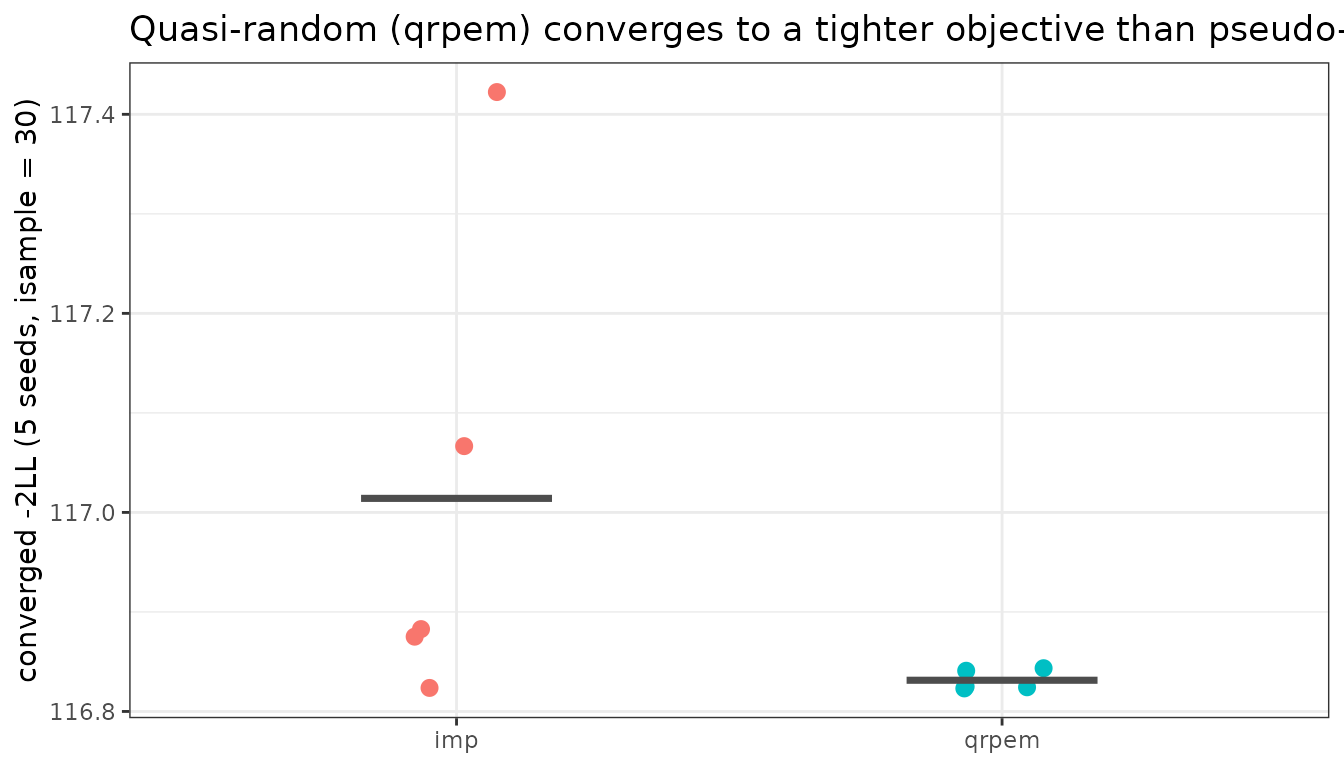

The qrpem objectives cluster tightly; the imp objectives scatter more than an order of magnitude wider for the same number of samples. In practice that means qrpem reaches a given precision with fewer importance samples – the reason it is a popular production EM method. (At the default isample = 300 both are already tight; quasi-random simply lets you use far fewer.)

Key parameters

All three methods share one control, impmapControl(); impControl() and qrpemControl() are thin wrappers over it. It also accepts every foceiControl() argument, since the MAP inner problem is the FOCEI one.

The ones you will actually change

isample (default 300) – importance samples per subject per iteration, NONMEM’s ISAMPLE. This is the master dial: it sets both the Monte-Carlo noise in the objective (as 1/sqrt(isample), or better under qr = TRUE) and essentially all the runtime, which is linear in it. Raise it when the objective trace is noisy, when the ESS fraction is low, or when you need a precise likelihood for model comparison. Lower it (with qr = TRUE) when iterating on an expensive model.

nIter (default 100) – the maximum number of EM iterations. This is a budget, not a target; hitting it is normal at default settings. Raise it if the objective trace is still trending rather than wobbling.

ctol (default NULL, i.e. 10^-sigdig = 1e-4) and nConvWindow (default 10) – the convergence test. ctol is compared against the mean absolute objective change over the trailing nConvWindow iterations, relative to the objective. Because that quantity is floored by Monte-Carlo noise, ctol and isample have to be chosen together: a tight ctol with a small isample can never converge. If you want converged = TRUE to be meaningful, either push isample up or set ctol to something comparable to the noise you can see in the trace.

covMethod (default "imp") – how standard errors are computed. "imp" takes a finite-difference Hessian of the importance-sampling objective over a fixed sample set (common random numbers), which keeps the finite-differencing well behaved. Alternatives "analytic", "r,s", "r", "s" compute the ordinary FOCEI covariance post-fit at the converged estimates; "" skips the covariance step entirely. One documented caveat: with covMethod = "imp" the variance of a tightly-determined random effect (an Omega diagonal) can be over-estimated, because the fixed samples barely span its prior variation – the theta standard errors match the Hessian-based FOCEI covariance. If the Omega standard errors look large, refit with covMethod = "analytic" to check.

impSeed (default 42) – base seed for the per-subject RNG streams. Results are reproducible and independent of the number of threads, which is worth knowing: you can change cores without changing the answer. Vary this to measure your own Monte-Carlo noise, as the seed study above does.

Checking the sampler is trustworthy: `impPsisK`

fit$env$impPsisK is a Pareto k-hat per subject – the tail index of that subject’s importance weights. Read it as:

k < 0.5 – reliable
0.5-0.7 – degrading
k > 0.7 – unreliable: those weights have infinite variance and the subject’s contribution is not trustworthy however good it looks elsewhere

This is worth checking because the other two statistics cannot detect the problem. xi and the Kish effective-sample fraction are both means over samples drawn from the proposal, so neither sees a tail the proposal rarely visits. On a three-ETA theophylline model, three of twelve subjects read k-hat above 0.7 (up to 1.13) while the median ESS fraction over all twelve is 0.96 – the efficiency statistic looks excellent on exactly the subjects whose weights are not trustworthy.

Tail trouble tends to track the number of random effects rather than the amount of data: the same data and structural model with a single ETA reads k-hat about -1.8 for every subject.

If impPsisK is above 0.7, more samples will not fix it – see df.

Proposal shape: `df` (and `auto`)

df (default 0) sets the proposal’s degrees of freedom: 0 is a multivariate normal, any positive value a multivariate t. This is the knob for a bad impPsisK, because it changes the proposal’s tails rather than its width – and tail weight, not width, is what makes importance weights well behaved. It is remarkably cheap: df = 20 cleared every failing subject on theophylline for 0.25% of the effective sample size.

auto (default TRUE) is NONMEM’s AUTO=1: pick df, isample and iaccept per subject rather than globally. It escalates df only for subjects whose k-hat says they need it and leaves the rest on the cheaper Gaussian, and it shifts sample budget from data-rich subjects to difficult ones.

The trade is measured: auto takes max k-hat from 2.44 to 0.49 and improves Omega accuracy by ~20%, at ~19% more Monte-Carlo noise on the objective. It is on by default because weights with infinite variance are a correctness problem – their error is unbounded in the worst case – while the extra noise is a bounded, measurable cost.

Set auto = FALSE to apply one global df, isample and iaccept to every subject. That is worth doing when you want the tightest possible objective on a model whose impPsisK values are already comfortably below 0.7, since there is no tail failure for the per-subject adaptation to repair.

Proposal tuning (rarely needed)

gamma (starting value 1.0, NONMEM’s ISCALE) inflates the proposal covariance. gamma = 1 means “use the Laplace covariance as-is”, which is optimal when the posterior really is Gaussian; values above 1 widen the proposal so it covers heavier tails. The importance weights correct for gamma, so changing it moves the variance of the estimates, never their expectation.

iaccept (default 0.4, NONMEM’s IACCEPT) is the target gamma is adjusted toward, and gammaRule chooses how:

"target" (default) is NONMEM’s rule – gamma is adjusted both ways until xi approximates iaccept, by at most 1.25x per iteration each way and clamped to iscaleMin/iscaleMax (defaults 0.1/10). Both bounds are reachable.
"floor" treats iaccept as a one-sided floor on the mean Kish effective-sample fraction instead: gamma is left at its efficient starting value while coverage is healthy and only ever inflated. Under it only iscaleMax can bind.

The tuned constants travel with the rule: choosing one also chooses its tuned nConvWindow (20 for "target", 10 for "floor"), because the target rule tracks a Monte-Carlo statistic and needs a longer window to average it out. An explicitly supplied value always wins.

Why "target" is the default. Tuned against tuned – each rule with its own constants, six seeds, isample = 300, RMSE against an isample = 6000 reference:

fixture	rule	theta RMSE	`Omega` RMSE	max k-hat	subjects k>0.7	converged
1 ETA	`"floor"`	0.00113	0.00193	-1.398	0.00	67%
1 ETA	`"target"`	0.00224	0.00130	-1.370	0.00	100%
3 ETA	`"floor"`	0.00187	0.00291	+0.604	0.33	100%
3 ETA	`"target"`	0.00176	0.00202	-0.429	0.00	100%

"target" wins every column at three ETAs, wins Omega RMSE and convergence at one, and is the only rule that adapts at all at eight ETAs – there "floor" leaves gamma pinned at 1.0 with xi at 1.35, a proposal far too narrow, because it watches the Kish fraction, which stays healthy while xi says otherwise. Its cost is theta RMSE on the one-ETA fixture and roughly twice the iterations.

That trade is the same one auto makes: weights with infinite variance are a correctness problem whose error is unbounded, while the extra Monte-Carlo noise is bounded and measurable.

Note "target" repairs the tail itself – it takes max k-hat from 0.836 to about -0.4 on the three-ETA fixture – so under the default the df ladder (see auto) is a secondary safety net rather than the primary remedy.

Choose "floor" when you want the proposal left at its efficient starting value – the tightest objective on a model whose impPsisK values are already comfortably below 0.7, where there is no tail to buy coverage for.

Sampling scheme (what `qrpem` turns on)

qr (default FALSE; TRUE under qrpemControl()) switches the draws to a Sobol quasi-random point set. qrShift (default TRUE) applies a random Cranley-Patterson shift per (iteration, subject), and qrRefresh (default TRUE) redraws that shift each iteration so residual quasi-random error averages out over the EM. Setting qrShift = FALSE gives a fully deterministic E-step with no RNG in the draw at all; qrRefresh = FALSE gives one shift per subject for the whole fit, which makes each EM iteration a deterministic map and produces the smoothest objective trace.

sir (default FALSE; TRUE under qrpemControl()) accelerates the non-mu / residual-error M-step by sampling-importance-resampling: the sensitivity Newton step uses sirSample equal-weight resampled points per subject (default max(25, isample/10)) instead of all isample weighted ones. This cuts the most expensive part of the M-step by roughly a factor of ten at essentially no cost in accuracy, because the resampled set already carries the weight information.

combSens (default TRUE) is a different M-step acceleration, and the two are complementary rather than alternatives. Without it (combSens = FALSE), a non-mu (structural or residual-error) theta’s d(f)/d(theta)/d(V)/d(theta) sensitivities are read from a second, dedicated model that re-solves every importance sample the E-step’s own inner-model solve had already produced value and eta-sensitivities for. combSens = TRUE instead carries those theta columns on the inner model itself, so with sir = FALSE (the default) the E-step’s own per-sample solve supplies the M-step’s Newton step directly – one ODE solve per sample instead of two. It defaulted to opt-in for one release while folding more sensitivity states into one coupled ODE system was still a live concern for a model with a non-mu structural theta; that concern turned out to be a genuine, unrelated bug rather than a property of combSens itself (see Does combSens change any of this?), and with the bug fixed combSens = TRUE/FALSE agree, so it is now the default.

Proposal family: `proposal`

df selects between a normal and a t proposal, but it cannot express every useful shape. proposal names the family directly. "auto" (the default) resolves to "t" when df > 0 and "normal" otherwise, so nothing about the historical df behaviour changes.

"normal" / "t" – the two families df already reached.
"laplace" – a spherical (Kotz-type) multivariate Laplace, f(x) ~ exp(-sqrt(x' S^-1 x)). Its exponential tail dominates the joint target’s, which for a bounded likelihood is at worst Gaussian, so the importance weights are bounded by construction – without having to guess a df, and without the effective-sample-size cost a low-df t pays. Its scale is covariance-matched (S = Sigma/(p+1)), so gamma, iscaleMin and iscaleMax keep the meaning they have for "normal".
"mixture" – a defensive scale mixture about the same mode, sum_k w_k N(mode, c_k gamma Sigma), set by propMixScale and propMixWeight. A broad component covers what a narrow one misses. Note this does not bound the weights: its widest component is still Gaussian-tailed. Use "laplace" when bounded weights are what you need.

All four are elliptical and share the MAP mode, which is what keeps the peak-normalised kernel exactly 1 at the mode – the property xi and both gamma controllers are built on. auto adapts df only on the normal/t axis: its ladder encodes “Gaussian” as df <= 0 and its constants were tuned against a Gaussian baseline, so a subject on "laplace" or "mixture" keeps its family while the isample budget reallocation still applies to it.

fit$env$impProposal reports the resolved family and fit$env$impPropInd the per-subject families actually used, so an auto escalation from normal to t is visible.

Scrambling the quasi-random points: `qrScramble`

A Cranley-Patterson shift randomises the Sobol set but leaves the correlation structure between the sequence’s dimensions intact. qrScramble permutes the digits instead and does break it: "owen" is a hash-based nested uniform (Owen) scramble, "lms" a linear matrix scramble with a digital shift. "none" (the default) keeps the historical behaviour.

What this is measured to buy, which is not what the theory suggested. The plausible story – a shift helps least where the sequence degrades first, so a scramble should help most with many random effects – is not what happens. The advantage is real but flat in dimension (1.79x on a smooth test integrand at one dimension, 1.53x at twelve), and it lands on the E-step integral rather than on the estimates: single-iteration IS -2LL RMSE 0.056 under "owen" against 0.080 unscrambled at three ETAs, while converged theta RMSE is unmoved at one ETA and worse at three, eight, and on a general-ll() model. At eight ETAs – the dimension where a scramble was expected to win – it is the worst of the three settings on theta and improves no k-hat.

That is why "none" is the default. Reach for "owen" when the number you care about is the reported importance-sampling objective (fit$env$impObj, say for comparing models by IS likelihood) rather than the parameter estimates: that integral is the one it measurably improves. The full table is in ?impmapControl.

Scrambling replaces the shift rather than composing with it, so qrShift is ignored when it is on; qrRefresh still decides whether the randomisation is redrawn each iteration. The scramble key is derived arithmetically from impSeed and the (iteration, subject, dimension) indices rather than drawn from the RNG, so it consumes no draws and the fit stays reproducible and independent of the thread count.

Burn-in: `nBurn`, `burnFreezeOmega`

The first EM iterations run under a proposal whose scale the controller has not yet adapted, and Omega’s update is the one that absorbs that – it is built from the conditional variances, which an over- or under-dispersed proposal estimates badly. nBurn runs that many settling iterations first, and burnFreezeOmega holds Omega at its starting value through them while the structural and residual-error thetas update normally.

Burn-in iterations are extra, not carved out of nIter, so raising nBurn never silently shortens a fit. Convergence is not tested until the whole trailing nConvWindow lies past the burn-in, so a frozen Omega cannot be mistaken for a settled one. Both default off.

MAP-assist period: `mapIter`

mapIter is the MAP-assist period: 1 (the default) re-centres the proposal at each subject’s MAP mode every iteration, k > 1 every kth, and 0 not at all after the startup MAP pass. The MAP search is the mu-referenced FOCEI inner problem and the dominant per-iteration cost of impmap, so raising it trades proposal accuracy for speed – worth doing once the population parameters move slowly enough that the mode barely shifts, and not before. A proposal centred away from the mode costs effective sample size, which impNeffFrac will show.

Skipping a MAP does not freeze the proposal centre: the M-step reseeds every subject’s eta with its conditional mean, so the centre still moves; it is the re-optimisation that is skipped. est = "imp" is a different thing and not the mapIter = 0 case – it also replaces the MAP-Hessian proposal covariance with the running conditional variance, so it never uses a MAP mode at all.

How it works, in plain terms

Everything above is enough to run these methods well. The rest of the article is the reference half: what the algorithm actually does, how it lines up with FOCEI and SAEM, and a step-by-step comparison with NONMEM.

The integral that has to be done

Every population model has one hard quantity in it. For subject i, the likelihood of that subject’s data requires averaging over all the values their random effects eta could have taken:

p(y_i) = integral  p(y_i | eta) * p(eta)  d(eta)

There is no closed form for this once the model is nonlinear, so every estimation method is really a strategy for handling this integral:

FOCEI replaces the integrand with the Gaussian that best matches it at its peak, and uses that Gaussian’s known area – the Laplace approximation. Fast and deterministic, but wrong by an unknown amount when the true integrand is skewed or heavy-tailed.
SAEM never evaluates the integral; it walks an MCMC chain through the posterior and averages parameter updates over iterations.
The imp family evaluates the integral numerically, by sampling.

Importance sampling, without the equations

The naive way to evaluate that integral by sampling would be to draw eta values from the population distribution p(eta) and average p(y_i | eta) over them. That works, but it is hopelessly wasteful: almost every draw lands somewhere the subject’s data says is implausible, contributing essentially nothing to the average. (NONMEM offers this as METHOD=DIRECT and notes it can need 10,000-300,000 samples per subject.)

Importance sampling fixes the waste with one idea: draw from a distribution that already looks like the answer, then correct for having done so.

One way to picture it: suppose you are estimating the average depth of a lake by dropping a probe at random points. Dropping uniformly over the whole map wastes most probes on the shallow edges. Instead, deliberately concentrate the probes where you believe the lake is deep – then, when averaging, down-weight each probe by how much more likely you were to drop it there. The bias you introduced by aiming is exactly cancelled by the weights, and you learn far more per probe.

The “where you believe it is deep” distribution is the proposal, q_i(eta). The correction is the importance weight

w = p(y_i | eta) p(eta) / q_i(eta)      [ what we want / what we sampled from ]

Two things fall out of the weighted samples at once, and this is the whole appeal of the method:

the average weight is an unbiased estimate of the integral p(y_i) – the subject’s marginal likelihood;
the weighted average of the samples is the subject’s conditional mean E[eta_i | y_i], and the weighted spread is the conditional variance – the quantities the EM update needs.

The EM loop

Each iteration does an E-step (compute expectations, with the parameters held fixed) and an M-step (update the parameters, with the expectations held fixed):

Build a proposal. For each subject, form a multivariate normal q_i aimed at that subject’s posterior. impmap finds the MAP mode and uses the inner Hessian as its covariance; imp re-uses the conditional mean and variance from the previous iteration. Both then inflate the covariance by a factor gamma so the proposal is a little wider than the posterior – deliberately over-dispersed, which keeps the weights from being dominated by a single lucky sample.
Draw isample points from q_i, independently for each subject. qrpem replaces the pseudo-random draw with a Sobol quasi-random point set.
Weight each point by the importance ratio above, and normalise the weights within the subject so they sum to 1.
Read off the E-step quantities: the subject’s marginal -2LL from the mean weight, and the conditional mean and variance from the normalised weighted samples.
M-step, part 1 – the mu-referenced fixed effects. For a plain tcl-plus-eta.cl parameter the EM update is just a mean shift: move tcl by the average conditional eta.cl and re-center the etas on zero. Where a covariate group is present, the group is updated by regression instead.
M-step, part 2 – everything else. Structural and residual-error parameters that are not mu-referenced are updated by a Newton step built from the importance-weighted score, using analytic d(f)/d(theta) and d(V)/d(theta) sensitivities from the rxode2 sensitivity model.
M-step, part 3 – Omega. The new Omega is the average, over subjects, of eta_i eta_i' + V_i: the spread of the individual estimates plus the average uncertainty in each. Elements not in the model are masked out and fix()ed variances are restored.

Repeat until the objective and the estimates stop moving. Because the samples are independent across subjects, the E-step is embarrassingly parallel, and the marginal likelihood comes out every iteration for free.

What `imp` and `impmap` actually change

Only step 1 differs, and it is a trade between cost and aim:

	`imp`	`impmap`
Proposal center	the subject’s conditional mean, carried over from the previous E-step	the subject’s MAP mode, re-found every iteration
Proposal covariance	`gamma` x the previous conditional variance (`gamma` x `Omega` on the first iteration)	`gamma` x the inverse inner Hessian at the mode
Cost per iteration	cheap – no mode search	a MAP search plus a Hessian per subject, every iteration
Aim	looser; needs more samples for the same precision	tighter; usually the more sample-efficient of the two
Fails when	the running mean has drifted somewhere unhelpful	the mode search is unstable (flat or multimodal posteriors)

Note that imp is not the same as sampling from the population distribution. It still aims at each subject individually; it just re-uses last iteration’s aim rather than paying for a fresh mode search. This is exactly the distinction NONMEM draws between METHOD=IMP and METHOD=IMPMAP.

How it maps onto other tools

NONMEM. imp and impmap are nlmixr2’s implementations of METHOD=IMP and METHOD=IMPMAP. See Appendix A for the step-by-step comparison.

Phoenix NLME (Certara). QRPEM is Phoenix’s flagship EM method, from Leary & Dunlavey. nlmixr2’s qrpem implements the published quasi-random parametric EM with SIR acceleration; Phoenix’s production code is proprietary and its exact details are not public, so the two are not guaranteed identical, but they share the defining ideas (Sobol importance samples, SIR-accelerated convergence). See Appendix C for a knob-by-knob comparison against the options Phoenix exposes.

FOCEI. FOCEI is a deterministic Laplace approximation of the marginal likelihood; the imp family is a Monte-Carlo evaluation of the same likelihood. They agree when the posterior is near-Gaussian and diverge when it is not – which is precisely when you want the importance-sampling number. FOCEI is faster and noise-free; the imp family is (asymptotically) unbiased, and reports both numbers so you can see the difference.

SAEM. SAEM is also an EM, but its E-step is an MCMC chain with stochastic-approximation (Robbins-Monro) averaging across iterations, and it does not produce the marginal likelihood directly. The imp family’s E-step uses independent importance samples and yields the likelihood every iteration. SAEM is exceptionally robust for difficult or multimodal problems; the imp family is efficient and self-certifying on the likelihood when a good proposal exists.

Aspect	FOCEI	SAEM	imp / impmap / qrpem
Marginal likelihood	Laplace approximation	Not direct (separate step)	Monte-Carlo importance sampling
E-step	Analytic conditional step	MCMC + stochastic approximation	Importance sampling (independent draws)
Reported objective	Laplace `-2LL`	Own convention	FOCEi `-2LL` (`objf`) plus the IS `-2LL` (`impObj`)
Character	Deterministic, fast	Stochastic, very robust	Stochastic, unbiased, parallel
Non-normal / nonlinear posteriors	Biased	Handles well	Handles well
External equivalents	NONMEM FOCEI; Phoenix FOCE	NONMEM SAEM; Monolix	NONMEM IMP/IMPMAP; Phoenix QRPEM
Sampling efficiency (this family)	–	–	`qrpem` > `impmap` > `imp`

Appendix A: nlmixr2 vs NONMEM, step by step

Equation numbers below refer to the NONMEM 7 Technical Guide (R.J. Bauer), section “Evaluating the Expectation step: Importance Sampling”. The derivation there is the reference implementation both tools are following, so the similarities run deep – the differences are mostly about how each step is executed rather than what it computes.

Two NONMEM sources, and what neither of them tells you

Before the step-by-step, three things about the source material, because they change how this comparison should be read.

The Technical Guide’s derivation is entirely Gaussian. Equations 1.65-1.104 build the proposal as a multivariate normal, scaled by gamma (ISCALE), with gamma “continually adjusted so that xi_i approximates IACCEPT”. The word DF does not appear. Read on its own, the guide gives the impression that widening a Gaussian is the only lever NONMEM has.

It isn’t. Bauer’s NONMEM Tutorial Part II (2019) documents what the guide omits: “When there are fewer data points than there are ETAs to be estimated (sparse data) or data are categorical, then DF (degrees of freedom) should be set to a nonzero number to use the t-distribution sampler and/or decrease the acceptance rate IACCEPT from the default value of 0.4 to about 0.2.” It also documents per-subject ISAMPLE, and AUTO=1, which “requests NONMEM to make decisions about IACCEPT, DF, and ISAMPLE for each subject”. That is a materially different method from the one the guide describes, and it is the one that matters for the non-Gaussian case.

Neither source publishes the numbers. NONMEM does not say what AUTO=1 actually picks – what DF it chooses, how it decides, or how it splits the sample budget. Only two concrete values appear anywhere: the nobs < neta trigger and IACCEPT ~ 0.2. So where this appendix quotes a number for nlmixr2 – df = 30, the k-hat thresholds, the budget rule, the 2/neta damping exponent, the 1.25x cap – those are nlmixr2’s own choices, tuned on measurements shown below, not reproductions of NONMEM’s internals. Treat any apparent numerical agreement with a NONMEM run as coincidence unless you have verified it.

Step 1 – Build the proposal density

NONMEM. For IMPMAP the proposal is centered at the MAP mode phi_hat_i with covariance gamma * (Omega^-1 + S_i^-1)^-1 – the inverse of the joint information at the mode (eqs. 1.67, 1.71). For IMP it is centered instead at the previous iteration’s conditional mean mu_pi with covariance gamma_i * Sigma_pi, the previous conditional variance (eq. 1.90). Whether a MAP estimation happens on a given iteration is governed by MAPITER and MAPINTER.

nlmixr2. Identical in structure. impmap takes the mode and the inner Hessian H_i from the mu-referenced FOCEI inner problem and uses gamma * H_i^-1; imp takes the running conditional mean and the previous E-step’s conditional variance V_i, using gamma * V_i, falling back to gamma * Omega on the first iteration where no V_i exists yet.

Same: the two proposals and the reason for each; the over-dispersion factor gamma. Different: nlmixr2 has no MAPITER/MAPINTER schedule. The choice is binary and made by est=: impmap re-MAPs on every iteration, imp on none (beyond the initial pass). The mode and Hessian come from nlmixr2’s FOCEI inner optimizer, so impmap inherits FOCEI’s inner tolerances and its handling of censored data.

Step 2 – Draw the samples

NONMEM. ISAMPLE pseudo-random multivariate normal draws per subject per iteration (r in the guide).

nlmixr2. isample draws, default 300, from a per-subject threefry stream seeded off impSeed and offset per (iteration, subject).

Same: the count and its role. Different: (a) nlmixr2 optionally draws a Sobol quasi-random point set instead (qr = TRUE, i.e. qrpem), optionally with a Cranley-Patterson shift; the technical-guide derivation of IMP/IMPMAP is entirely pseudo-random. (b) nlmixr2’s stream is indexed per (iteration, subject) rather than drawn from one global stream, which makes a fit bit-identical regardless of thread count. (c) A proposal sample whose ODE solve fails is given weight zero and dropped from the weighted moments rather than aborting the subject.

Step 3 – Form the importance weights

nlmixr2. The same log-ratio, computed with the constant terms factored out of the per-sample loop: the per-sample part is -(negative log joint density) + (1/(2 gamma)) d' H_i d, and the constants -0.5 log|Omega| + (n_eta/2) log gamma - 0.5 log|H_i| are added once. Weights are formed with a max-subtraction (exp(q - max q)) for numerical stability.

Same: the quantity, exactly. Different: only the arrangement and the log-sum-exp stabilization.

Step 4 – Individual likelihood and effective sample size

NONMEM. xi_i = mean(u_(k)i) (eq. 1.79), L_i = -log(xi_i) (eq. 1.80), objective L = sum_i L_i (eq. 1.81). The reported Neff. is (r/m) sum_i F_i xi_i (eq. 1.94), where F_i corrects for a proposal centered at the conditional mean rather than the mode, and is fixed at 1 for IMPMAP.

nlmixr2. L_i = -(logMeanExp + C_i) with the same constants, and the importance-sampling objective is sum_i 2 L_i, stashed as fit$env$impObj. The effective sample size is the Kish ESS, 1 / sum_k z_k^2, reported as a fraction of isample in fit$env$impNeffFrac.

Same: the individual likelihood and the summed objective. Different: (a) the ESS definitions differ – Kish ESS versus NONMEM’s F_i-corrected mean weight. Both equal isample when proposal and posterior coincide, and both are read the same way (higher is better), but the numbers are not interchangeable. nlmixr2 does not compute NONMEM’s “fitness” statistic (eq. 1.96). (b) What gets reported as the fit’s objective differs. NONMEM reports the importance-sampling objective. nlmixr2 reports the FOCEi objective at the converged EM estimates as fit$objf and keeps the importance-sampling value in fit$env$impObj; compare impObj against a NONMEM IMP objective, not objf – and check the constant convention on both sides before reading anything into a small difference.

Step 5 – Conditional moments

NONMEM. Normalised weights z_(k)i = u_(k)i / sum_k u_(k)i (eq. 1.82), conditional mean mu_i = sum_k z_(k)i phi_(k)i (eq. 1.84), conditional variance B_i = sum_k z_(k)i (phi_(k)i - mu_i)(phi_(k)i - mu_i)' (eq. 1.85).

nlmixr2. Identical.

Same: everything.

Step 6 – M-step for the mu-referenced fixed effects

NONMEM. A Gauss-Newton step on theta from the score g_theta = sum_i (d mu_i / d theta)' Omega^-1 (phi_bar_i - mu_i) and information H_theta = sum_i (d mu_i/d theta)' Omega^-1 (d mu_i/d theta), giving theta_hat = theta + lambda H_theta^-1 g_theta (eqs. 1.86-1.88).

nlmixr2. Split by structure. A simple mu-referenced intercept (a theta that is the population mean of an eta, no covariates) is updated by its exact EM fixed point – shift the theta by the mean conditional eta and re-/sscenter the etas – rather than by a Newton step. Covariate mu-groups go through a regression update.

Same: the fixed point being sought. Different: the route to it. For the no-covariate case the mean shift is the solution of NONMEM’s Newton system in one step, so this is a simplification rather than a different answer.

Step 7 – M-step for non-mu and residual parameters

NONMEM. Finite differences on the whole individual likelihood, one extra likelihood evaluation per non-mu theta per sample (eqs. 1.97-1.99); the Hessian is the outer product of the per-subject gradients (eq. 1.102). SIGMA parameters get a shortcut that avoids re-solving the ODE, and a THETA that affects only the residual variance can be flagged S in GRD= to get the same shortcut; otherwise the guide’s advice is to mu-model whatever you can, because each non-mu parameter costs n_theta * r extra likelihood evaluations.

nlmixr2. An importance-weighted Newton step built from analytic symbolic sensitivities – d(f)/d(theta) and d(V)/d(theta) from the rxode2 sensitivity model, including exact partials for censored (M2/M3/M4) points – with a Gauss-Newton information matrix.

Same: the target (a Newton step on the IS-weighted score for the non-mu block). Different: this is the largest algorithmic difference. nlmixr2 does no finite differencing here, so there is no GRD=-style annotation to get right, no step-size sensitivity, and no n_theta-fold multiplication of the solve cost. qrpem’s sir = TRUE shrinks this step further by resampling to sirSample equal-weight points – an acceleration with no NONMEM IMP/IMPMAP counterpart.

Step 8 – M-step for Omega

NONMEM. Omega_hat = (1/m) sum_i sum_k z_(k)i (phi_(k)i - mu_i)(phi_(k)i - mu_i)', equivalently the sample variance of the conditional means plus the mean conditional variance (eqs. 1.66, 1.89).

nlmixr2. The same: Omega = (1/m) sum_i (eta_i eta_i' + V_i) over the re-centered etas, then masked to the elements actually estimated in the model, with fix()ed rows and columns restored to their starting values.

Same: the estimator. Different: the structural mask and fix() handling are nlmixr2-side bookkeeping for its ini({}) block; NONMEM does the equivalent through $OMEGA ... FIX and the block structure.

Step 9 – Adapting the proposal scale

NONMEM. gamma is continually adjusted so that xi_i approximates IACCEPT, bounded by ISCALE_MIN and ISCALE_MAX. The subscript in eq. 1.90 (gamma_i) indicates this is done per subject.

nlmixr2. gammaMethod chooses shared vs per-subject, and gammaRule chooses the law for the shared one:

"global" – one shared gamma. Under gammaRule = "target" (the default) it is adjusted two-sided until xi approximates iaccept, which is NONMEM’s rule; under gammaRule = "floor" it is a one-sided floor on the mean Kish ESS fraction, which is not.
"individual" – per-subject gamma_i, adapted two-sided toward iaccept on that subject’s own xi_i, which is NONMEM’s rule per subject.
"auto" (default) picks between shared and per-subject on the model’s distribution.

Same: the role of gamma, the names and meaning of IACCEPT/ISCALE_MIN/ ISCALE_MAX, the per-subject option, and the fact that the weights correct for gamma so it affects variance and not expectation.

Different: the guide gives no update formula, so nlmixr2’s is its own. It is gamma_i * (xi_i/iaccept)^p with p = 2/neta. That exponent is not a tuning constant: for a Gaussian posterior xi = gamma^(-neta/2) inverts exactly, so p = 2/neta is the analytic solve. A fixed exponent is what needs justifying, and it fails – with p = 1/2 the error multiplier is 1 - neta/4, which is -1 at neta = 8, giving a period-2 limit cycle that never settles (measured: gamma oscillating 1.30/1.22/1.30/1.22 with lag-1 autocorrelation -0.99, so the fit can never meet its own stability gate).

What the target costs. Driving xi onto IACCEPT = 0.4 deliberately over-disperses a proposal that may already fit: on theophylline it costs effective sample size (0.96 -> 0.70) and adds Monte-Carlo noise to the objective.

That noise is why the two rules carry different tuned constants. The target rule needs a longer convergence window (nConvWindow 20 against 10), and its objective gate measures the drift of the window mean rather than the mean absolute change between iterations – the latter is a noise measure whose floor the wider proposal raises, so it would never settle however converged the fit was. With each rule measured on its own constants the target wins on accuracy as well as on the tail (see Proposal tuning); the ESS cost is real but is not the whole ledger.

Step 9b – Proposal shape: the t sampler (`DF`)

This step has no counterpart in the Technical Guide at all; it comes entirely from the tutorial, and it is the most consequential difference in the appendix.

NONMEM. DF switches the proposal from a multivariate normal to a multivariate t. The tutorial’s advice is to set it nonzero for sparse (nobs < neta) or categorical data. It does not say which value.

nlmixr2. impmapControl(df=), with 0 meaning Gaussian. The kernel becomes (1 + d'Hd/(gamma*df))^(-(df+p)/2) and the normalizer gains (p/2)log(df/2) + lgamma(df/2) - lgamma((df+p)/2), which tends to 0 as df grows, recovering the Gaussian exactly.

Why it matters more than gamma. gamma can only make a Gaussian proposal wider; it cannot give it heavier tails. When the target’s tails are heavier than the proposal’s, the importance weights have infinite variance – and neither xi nor the Kish ESS can see it, because the offending mass sits where the proposal rarely lands. Measured on plain theophylline, a transformably-normal model with 11 observations per subject:

subject	Pareto k-hat	`xi`	ESS frac	verdict
1	2.60	0.98	1.00	unreliable
5	0.68	0.96	0.99	degrading
10	1.28	0.96	0.99	unreliable
others	0.0-0.5	~1.0	~1.0	ok

Two of twelve subjects have infinite-variance weights while both in-sample statistics read healthy for those same subjects. It is not a small-sample artifact: max k-hat grows with more draws (2.49 -> 3.31 -> 3.76 at isample 300 -> 1000 -> 4000), which is what a genuine heavy tail does.

Three remedies compared on that fixture:

approach	max k-hat	subjects k>0.7	cost
Gaussian, `isample = 300`	1.61	4	baseline
Gaussian, failing subjects at `isample = 3000`	3.28	1	10x samples
t proposal, `df = 20`	-0.58	0	0.25% of ESS

More samples treats the symptom and can make matters worse – extra draws reach further into the tail the proposal misses. Only a heavier tail treats the cause, and it is nearly free.

Same: the existence and purpose of a t proposal for sparse/categorical data. Different: every number. NONMEM publishes no DF value; nlmixr2’s auto enters at df = 30, chosen from a sweep in which df = 30 clears the failure for a 7% RMSE cost while df = 8 costs 3x for no extra tail benefit.

Step 9c – `AUTO`: per-subject `DF`, `ISAMPLE` and `IACCEPT`

NONMEM. AUTO=1 “requests NONMEM to make decisions about IACCEPT, DF, and ISAMPLE for each subject”, adapting ISAMPLE when there are “many ETAs or the objective function has large stochastic fluctuations”. The tutorial warns it “may result in lack of stochastic reproducibility”.

nlmixr2. impmapControl(auto=TRUE) implements the same three levers, and adds a fourth signal NONMEM does not have – Pareto k-hat – because the documented triggers turn out to be necessary but not sufficient: on a multi-ETA theophylline model neither nobs < neta nor “categorical” fires, yet subjects still fail. So df is escalated on k-hat severity (k>1 -> 20, k>0.7 -> 30), one-way. Escalation is deliberately not reversed: once a t proposal is working k-hat drops because it is working, so relaxing on a low k-hat walks straight back into the failure.

Both rungs come from the sweep in Appendix B, which also shows where escalation does not help.

isample is allocated proportional to inverse effective-sample fraction within a fixed budget, so data-rich subjects fund the difficult ones (measured on a mixed design: rich subjects 289-299 draws, sparse 300-329, total preserved).

Same: the three levers and their triggers. Different: all the numbers, the k-hat signal, and reproducibility – nlmixr2’s auto stays seeded and thread-count independent.

What it costs. Against a high-accuracy reference (isample = 8000), over 8 seeds on theophylline with 3 ETAs – a 1-ETA model has no tail failure to fix, so it shows nothing either way, see Appendix B:

	objective RMSE	max k-hat	subjects k>0.7	`Omega` RMSE
`auto = FALSE`	0.0113	0.941	2.38	0.00406
`auto = TRUE`	0.0165	0.571	0.25	0.00301

auto fixes the tail behaviour and estimates Omega about 26% more accurately, at roughly 46% more Monte-Carlo noise on the objective. It is on by default: infinite-variance weights are a correctness problem whose error is unbounded in the worst case, whereas the added noise is bounded and measurable. auto = FALSE applies one global df, isample and iaccept to every subject, which is the right choice when fit$env$impPsisK is already comfortably below 0.7 everywhere and you want the tightest objective you can get.

Two caveats worth reading before relying on it, both measured in Appendix B. If you already know the whole model is heavy-tailed, a global df gives a better objective than auto – but it costs 75% more objective RMSE on a model that did not need it, which is why it is not the default. And on subjects with fewer observations than random effects auto makes matters worse rather than better, because there the heavy tail is structural and no proposal can repair it.

Step 10 – Convergence

NONMEM. A statistical test over trailing iterations, configured through the CTYPE family of $EST options.

nlmixr2. A windowed test over the last nConvWindow iterations requiring three conditions simultaneously: the mean absolute relative objective change is below ctol; no parameter has drifted by more than 2% in net relative terms across the window; and gamma has stopped adapting. Missing any one leaves fit$env$impConverged at FALSE and the fit runs to nIter.

Same: windowed rather than single-iteration testing, and the recognition that a Monte-Carlo objective needs averaging before it can be tested. Different: the specific gates. In particular the parameter-drift and gamma-stability gates have no direct NONMEM analogue, and, as shown above, the default ctol is tight relative to the Monte-Carlo noise at isample = 300, so converged = FALSE is common and benign.

Step 11 – Standard errors

NONMEM. A separate $COV step after estimation, with its own method options.

nlmixr2. covMethod = "imp" (the default) computes a Monte-Carlo observed information: at the converged estimates it redraws one fixed sample set and takes a finite-difference Hessian of the importance-sampling -2LL over the thetas and the parameterized Omega elements. Because the same samples are reused for every perturbation (common random numbers) the reweighted objective is a smooth deterministic function of the parameters, so the finite differences are well behaved. Alternatively the ordinary FOCEI covariance can be computed post-fit (covMethod = "analytic", "r,s", "r", "s").

Same: the idea of an importance-sampling-based covariance for an importance-sampling fit. Different: the common-random-number FD Hessian is nlmixr2’s construction, and it comes with the documented caveat that a tightly-determined Omega diagonal can have its variance over-estimated. Falling back to the FOCEI covariance is a one-argument change.

Other differences worth knowing

Mixture models. Both support mixtures, but the M-step for the mixing proportions differs: nlmixr2 uses the mean-posterior EM update (the proportions become the average responsibilities), because a full Newton step on NONMEM’s Gauss-Newton score for the proportions overshoots to the simplex boundary and collapses a component.
Mu-referencing. NONMEM strongly recommends mu-modeling for efficiency but permits non-mu thetas at a documented cost. nlmixr2 requires mu-referencing for the imp family (muModel = "lin"), and handles non-mu structural and residual parameters through the analytic-sensitivity step of Step 7 rather than through finite differences.
Parallelism. NONMEM parallelises across subjects via MPI/$PARALLEL. nlmixr2 parallelises the E-step and the sensitivity half of the M-step with OpenMP over subjects, and, as noted, guarantees the result does not depend on the thread count. The score accumulation is deliberately kept serial so the sum is bit-identical run to run.

Appendix B: what `auto` was tuned on

The df ladder in Step 9c is nlmixr2’s own – neither NONMEM source publishes a DF value, a threshold, or anything resembling a tail diagnostic – so it has to stand on measurement. This appendix records that measurement so the numbers are reproducible rather than asserted.

The code below is not run when this article builds; the tables are its recorded output.

Is the diagnostic trustworthy?

Everything below steers on Pareto k-hat, so the first thing to establish is that a low k-hat means what it claims. On plain theophylline every subject reads about -1.8, which is an unusually clean result and worth checking rather than assuming: genuinely light tails and a collapsed, near-uniform weight vector both drive k-hat down, and only one of those is good news.

Raising isample 20-fold is the test. It moves the objective by 0.037 (173.708 -> 173.671) and leaves the effective-sample fraction (0.536 -> 0.534) and k-hat (-1.46 -> -1.50) essentially unchanged. Had the weights collapsed, the cheap fit would have been biased and the reference would have pulled away from it. The tails really are light, so k-hat can be trusted as the steering signal.

It also means theophylline with one ETA does not exercise auto at all, so it is the wrong model to tune on.

Which models still stress the sampler

Run with auto = FALSE, isample = 300, nIter = 12, impSeed = 42:

model	subjects	max k-hat	k > 0.7	median ESS fraction
theophylline, `linCmt()`, 1 eta	12	-1.46	0/12	0.54
theophylline, `linCmt()`, 3 etas	12	1.13	3/12	0.96
sparse, 2 obs/subject, 3 etas (`nobs < neta`)	12	0.97	5/12	0.68
Poisson, 3 obs/subject, 1 eta	20	-1.45	0/20	0.54
theophylline + t(2) outlier contamination	12	0.91	3/12	0.96

The driver is the number of ETAs, not the data: identical data and structural model, 1 eta gives max k-hat -1.46 and 3 etas gives 1.13. This matches the tutorial’s “many ETAs” language, and it is why the tuning fixture is the 3-eta model.

Note also that the tutorial’s categorical trigger and k-hat disagree: the Poisson fixture fires the documented trigger while its tails are entirely healthy (max k-hat -1.45). The two signals are tested separately for that reason.

The `df` sweep

Theophylline with 3 ETAs, 8 seeds, RMSE against an isample = 8000 reference (reference max k-hat 0.548, i.e. the reference itself is sound):

`df`	objective RMSE	`Omega` RMSE	max k-hat	subjects k > 0.7
0 (Gaussian)	0.0113	0.00406	0.941	2.38
30	0.0095	0.00281	0.593	0.25
20	0.0097	0.00255	0.484	0.12
12	0.0105	0.00224	0.405	0.00
8	0.0116	0.00223	0.273	0.00

The objective RMSE is minimised at df = 30 and degrades past it – df = 8 is worse than using no t proposal at all – while the tail index and Omega continue to improve. That trade-off is what fixes the ladder at 30 and 20.

There is no rung above that. Nothing measured here reaches k-hat 2 (the sweep peaks at 1.13, and the sparse fixture below at 1.07), so a heavier rung would be guesswork on an unobserved regime; and where df = 12 can be measured it costs objective accuracy for a marginal Omega gain. If you do meet a model whose k-hat sits above 2, set df yourself rather than expecting auto to invent a value for it.

Where escalation does not help, and what is done about it

Some heavy tails are not the proposal’s fault. On a deliberately sparse fixture (2 observations, 3 ETAs – the tutorial’s own definition of sparse) no df moves max k-hat off about 1.07, and the reason is visible in the reference: at isample = 8000 that fixture still reads max k-hat 0.794. With fewer observations than random effects the individual posterior is not identified, so the heavy tail is structural, and a heavier proposal cannot repair what the data did not determine.

Applying the tutorial’s nobs < neta rule there makes every number worse. So that half of the trigger is not applied on its own: sparsity alone does not assign a t proposal, and an escalation that fails to improve k-hat within two iterations is withdrawn and the samples given back.

on the sparse fixture	objective RMSE	`Omega` RMSE	max k-hat	subjects k > 0.7
no adaptation	0.1517	0.02379	1.065	3.88
global `df = 30`	0.1666	0.02695	1.075	5.00
`autoNonmemSparse = TRUE` (the tutorial’s rule)	0.2059	0.03163	1.088	4.88
`auto` as shipped	0.1020	0.01838	1.020	4.62

The gated default gives the best objective, the best Omega and the least severe worst tail – and beats doing nothing at all, because it keeps the k-hat escalation and the budget reallocation where those help while withdrawing only the escalation that measurably does not.

The columns it does not lead are the count of subjects above 0.7 (4.62 against 3.88 for no adaptation) and, marginally, the worst tail (1.020 against 1.065). That is not a contradiction: escalation redistributes where the weight sits, so slightly more subjects sit marginally above the threshold. On a fixture whose failure is structural, no method drives that count down – the reference at isample = 8000 still reads 0.794.

Two things follow. First, when reading fit$env$impPsisK, k > 0.7 on a subject with fewer observations than random effects is telling you about the model, not about the sampler; no sampler setting will fix it. Second, this is the one place the measurement and the NONMEM tutorial pull in different directions, since the tutorial recommends DF precisely for nobs < neta. NONMEM’s own testing is not published and was not done on these models, so impmapControl(autoNonmemSparse = TRUE) restores the documented rule unchanged for anyone whose own measurements come out the other way.

Both halves matter, and gating the trigger on its own is not enough. Objective RMSE on the sparse fixture, by what is switched on:

	objective RMSE
`autoNonmemSparse = TRUE` (tutorial rule applied)	0.2059
gate the trigger, never withdraw (`autoDfPatience = 0`)	0.1807
`auto = FALSE` (no adaptation at all)	0.1517
gate the trigger and withdraw (shipped)	0.1020

Gating alone still loses to simply turning auto off; the withdrawal is what turns it into a win.

autoDfPatience sets how many consecutive non-improving iterations are tolerated before an escalation is withdrawn (0 never withdraws). Swept over 0, 1, 2, 3 and 5, 8 seeds:

patience	sparse obj RMSE	3-ETA obj RMSE	3-ETA `Omega` RMSE	3-ETA k>0.7
0	0.1807	0.01654	0.00301	0.25
1	0.1874	0.01418	0.00271	0.50
2 (default)	0.1020	0.01588	0.00184	0.38
3	0.1287	0.01654	0.00301	0.25
5	0.1827	0.01654	0.00301	0.25

2 is the sparse optimum and the curve rises either side of it. It is not the best objective on the 3-ETA fixture (1 is, 0.01418 against 0.01588), but 1 has the worst tail of any setting on every fixture (subjects above 0.7: 0.50, 0.38 and 4.50), because on fixtures where escalation genuinely helps, withdrawing that eagerly retracts proposals that were working. Tail behaviour is weighted higher for the same reason auto is on at all: weights with infinite variance are a correctness problem whose error is unbounded, while Monte-Carlo noise is bounded and measurable.

Note that patience interacts with nIter: at 3 and 5 the counter never accumulates inside a 12-iteration fit on a fixture whose k-hat does improve, which is why those rows are identical to switching withdrawal off. A longer fit will withdraw where a short one does not.

Why `auto` rather than a global `df`

If a t proposal helps, why adapt per subject at all instead of just setting df globally? Because a global df is only free on models that need it. Three methods over five fixtures, 8 seeds each, against per-fixture isample = 8000 references:

A – auto = FALSE, df = 0: plain Gaussian, no adaptation
B – auto = FALSE, df = 30: one global t proposal for everybody
C – auto = TRUE: per-subject df/isample/iaccept

fixture		A	B (global `df`)	C (`auto`)
theophylline, 1 eta (no tail problem)	obj RMSE	0.1091	0.1908	0.1148
	`Omega` RMSE	0.00117	0.00203	0.00118
Poisson (no tail problem)	obj RMSE	0.00525	0.00373	0.00341
	`Omega` RMSE	0.01329	0.01146	0.01072
theophylline, 3 etas (tail problem)	obj RMSE	0.01132	0.00952	0.01588
	`Omega` RMSE	0.00406	0.00281	0.00225
	subjects k>0.7	2.38	0.25	0.38
outlier-contaminated (tail problem)	obj RMSE	0.07680	0.04440	0.05223
	`Omega` RMSE	0.00817	0.00817	0.00735
	subjects k>0.7	2.50	0.12	0.12

(C here is auto as shipped, i.e. with the sparsity gate of the previous section. On the sparse fixture, which has no counterpart above because neither A nor B addresses it, C reads 0.1020 / 0.01838.)

Read the top two rows first. On a one-ETA model with no tail problem at all, a global df = 30 costs 75% more objective RMSE and 73% more Omega RMSE for no benefit whatsoever – both k-hats are already about -1.4 with nothing failing. auto costs about 5% there, and on the Poisson fixture it is the best of the three.

On the two fixtures that do have a tail problem, a global df gives the better objective (0.0095 vs 0.0165, and 0.0444 vs 0.0519) while auto gives the better tail and Omega. So a global df is the better choice once you already know your model is uniformly heavy-tailed – and that is exactly the thing you cannot know without having run something like this first.

That asymmetry is why auto is the default and df = 0 is its companion default: auto is close to free when it is not needed and effective when it is, whereas a global df is effective when needed and expensive when not.

# The harness that produced the tables above.  Not run during the article build.
mTheo3 <- function() {
  ini({tka <- 0.45; tcl <- 1; tv <- 3.45
       eta.ka ~ 0.3; eta.cl ~ 0.1; eta.v ~ 0.1; add.sd <- 0.7})
  model({ka <- exp(tka + eta.ka); cl <- exp(tcl + eta.cl); v <- exp(tv + eta.v)
         linCmt() ~ add(add.sd)})
}
run1 <- function(model, data, isample, df, seed, auto = FALSE, nIter = 12L) {
  fit <- nlmixr2(model, data, "impmap",
                 impmapControl(print = 0L, nIter = nIter, isample = isample,
                               df = df, covMethod = "", auto = auto,
                               impSeed = seed))
  k <- fit$env$impPsisK
  list(objf = as.numeric(fit$objf), omega = diag(fit$omega),
       maxK = max(k, na.rm = TRUE), nAbove = sum(k > 0.7, na.rm = TRUE))
}
ref <- run1(mTheo3, nlmixr2data::theo_sd, 8000L, 0, 42L)
for (df in c(0, 30, 20, 12, 8)) {
  rs <- lapply(1:8, function(s) run1(mTheo3, nlmixr2data::theo_sd, 300L, df, s))
  ob <- vapply(rs, function(z) z$objf, 1)
  om <- do.call(rbind, lapply(rs, function(z) z$omega))
  cat(sprintf("df=%-3g objRMSE=%.4f omRMSE=%.5f maxK=%.3f k>0.7=%.2f\n", df,
              sqrt(mean((ob - ref$objf)^2)),
              sqrt(mean((sweep(om, 2, ref$omega))^2)),
              mean(vapply(rs, function(z) z$maxK, 1)),
              mean(vapply(rs, function(z) z$nAbove, 1))))
}

Does `combSens` change any of this?

combSens (see Sampling scheme) changes only how the M-step’s non-mu theta-sensitivity gradient is computed – it never touches the E-step’s importance weights, which is what auto’s df/k-hat tuning steers on. So in principle it should not interact with any number in this appendix at all. That is worth checking rather than assuming, though, because folding the theta-sensitivity states into the SAME coupled ODE system as the eta sensitivities restructures the compiled inner model, which can move floating-point results by a small amount when a non-mu theta is structural (enters an ODE state directly) rather than purely residual-error – nlmixr2est’s own impmapControl(combSens=) documentation records this (confirmed on a one-ETA fixture where tka/tv are non-mu structural thetas, not the fixtures used here).

Every fixture the df/auto sweep above ran on – theophylline (1 and 3 ETA), the sparse fixture, and the Poisson fixture – has at most one non-mu theta, and it is always the residual-error add.sd (Poisson has none at all). A sigma-only non-mu theta needs no ODE sensitivity state: its sensitivity is purely algebraic, so there is nothing for combSens to fold into the shared ODE system. Re-running the mTheo3 and sparse-fixture grids with combSens = TRUE confirms it directly rather than by inference – every point checked (2-3 seeds each; every seed matched to the same precision, so one representative row is shown per configuration):

fixture	`df`	`auto`	`objf` (`combSens=FALSE`)	`objf` (`combSens=TRUE`)
theophylline, 3 ETA	0	`FALSE`	116.83403482	116.83403482
theophylline, 3 ETA	30	`FALSE`	116.83811796	116.83811796
theophylline, 3 ETA	0	`TRUE`	116.84654942	116.84654942
theophylline, 3 ETA	30	`TRUE`	116.83675595	116.83675595
sparse, `autoDfPatience = 0`	–	`TRUE`	25.71803423	25.71803423
sparse, `autoDfPatience = 2` (default)	–	`TRUE`	25.81800226	25.81800226

Max k-hat matched to the same four decimals on every row too (not shown), and odeSwapInfo_()$impThetaSensHarvestN confirmed the harvested M-step path was actually engaging under combSens = TRUE throughout – this is a checked equivalence, not a case where the new path silently declined to run.

Verdict: the golden ratios stand. df = 30/20/12/8, the k-hat breakpoints, autoDfPatience = 2, gammaRule = "target", and every other number in this appendix were tuned on, and remain exactly reproduced by, models combSens cannot perturb. Nothing here needed re-tuning, and none of auto’s defaults changed.

Update: the structural-theta discrepancy was a real bug, now fixed, not a combSens floating-point artifact. Chasing the caveat above (a one-ETA theophylline fixture with tka/tv as non-mu structural thetas) down to its source found that impmap’s inner Hessian – which builds the importance proposal – was reading a stale cached Jacobian from linCmtB() on that fixture, regardless of combSens. Several compiled models share one solve pool (nlmixr2est’s odeSwap), and linCmtB()’s Jacobian cache is gated by a process-global (rx->ndiff) that the pool’s per-individual solve entry point never restored for the peer actually being solved – so a solve could read a Jacobian shaped for a different peer’s structural-parameter set. The resulting proposal was artificially wide, which masked a real heavy tail as healthy (Pareto k-hat about -1.5) rather than actually being healthy (k-hat about 2.9 once the correct Jacobian is used). This is now fixed (nlmixr2est’s per-individual solve entry point restores each peer’s own ndiff before every solve), verified to make combSens = TRUE/FALSE agree on that fixture too, and is why combSens now defaults to TRUE: it exists for models with a non-mu structural theta, and the fix makes it correct there.

One consequence worth flagging for anyone who has treated a one-ETA, low-tail-failure fixture as a “does AUTO cost anything when nothing needs fixing” reference (as this article’s own package tests once did): if the model has a non-mu structural theta, a “healthy” k-hat measured before this fix may not have been healthy at all. Re-measure impPsisK after upgrading rather than trusting an old reading for such a model.

Appendix C: nlmixr2 vs Phoenix QRPEM, option by option

Phoenix NLME exposes a set of “Advanced Options for QRPEM only” in its model executor. That list is the closest thing to a public specification of what Phoenix’s QRPEM can be told to do, so it is a fair checklist to hold qrpem against – with one caveat stated up front, and meant literally: the option names tell you what Phoenix exposes, not what it computes. The algorithm behind each checkbox is not published. Nothing below should be read as a claim that the two implementations agree numerically; where the underlying method is genuinely not public, this article says so rather than guessing.

Phoenix option	nlmixr2 equivalent
MAP Assist	`est = "impmap"` (on) vs `est = "imp"` (off)
Periodicity for MAP Assist	`mapIter`
Number of Sample Points	`isample` – and ours also accepts a per-subject vector
Acceptance Ratio	`iaccept` (see the default note below)
Importance Sampling Distribution: MVN	`proposal = "normal"`
Importance Sampling Distribution: MVT	`proposal = "t"`
Importance Sampling Distribution: MVL	`proposal = "laplace"`
Importance Sampling Distribution: Mixture-2 / -3	`proposal = "mixture"`, `propMixScale`/`propMixWeight` of length 2 or 3
Number of Degrees of Freedom	`df`
Quasi-Random Scrambling Method	`qrScramble` (see below)
Number of SIR Samples	`sirSample`
Number of Burn-in Iterations	`nBurn`
Frozen Omega during Burn-In	`burnFreezeOmega`
MCPEM (Monte-Carlo instead of quasi-random)	`qr = FALSE`
Run All Requested Iterations	`nConvWindow = 0` disables the convergence test

Four places where the correspondence is a mapping rather than a match:

Scrambling. Phoenix offers None / Owen / Tezuka-Faure. nlmixr2 offers "none" / "owen" / "lms". "lms" is named for the method – Matousek / Tezuka linear matrix scrambling – and not after Phoenix’s label, because “Tezuka-Faure” is not published in enough detail to claim we reproduce that particular variant. Both of ours are applied to the generator’s output digits rather than to its direction numbers, which is legitimate for both: a Sobol point is a GF(2)-linear image of the direction numbers, so a linear scramble commutes with generation, and a nested digit permutation is defined on the digits however they were produced.

Acceptance ratio. Phoenix documents a default of 0.1 and describes lowering it as broadening the proposal. nlmixr2’s iaccept defaults to 0.4, which is NONMEM’s IACCEPT convention, and it is the target the two-sided gammaRule adapts toward rather than a threshold. The two numbers are not on the same scale and should not be transferred between programs.

SIR samples. Phoenix documents a default of 10 per subject; nlmixr2 uses max(25, isample/10). Ours is a floor-plus-fraction because the resampled set also has to remain usable for the Pareto k-hat diagnostic, which a set of 10 does not.

Mixture proposals. Phoenix names “Mixture-2” and “Mixture-3” without saying what the components are. nlmixr2 implements a defensive scale mixture about the shared MAP mode. That choice is not arbitrary: sharing the mode is what keeps the mixture’s peak density closed-form, and therefore keeps the peak-normalised kernel exactly 1 at the mode – the property qCenter, xi and both gamma controllers depend on. A mixture with per-component locations would break all four at once.

Why the defaults are what they are

Every capability added for these methods ships off by default, and the fits you would have got before they existed are unchanged. The one exception, combSens, is argued above. That was the starting policy, and the measurements below are why it is also the finishing one. The harness is design/qrpem/qrpem-options-bench.R: four fixtures (1, 3 and 8 ETAs plus a general-ll() model), 8 seeds at isample = 300, scored against an isample = 8000 reference.

The single most useful thing in that table is not any individual number, it is which fixture is which. Three of the four never fail: no subject exceeds Pareto k-hat 0.7 under any setting, because auto’s df ladder and gammaRule = "target" already keep them healthy. Only the 8-ETA warfarin PK/PD fit has a sampler that actually struggles (2.1 subjects over 0.7 under the default). So a proposal whose selling point is bounded weights has nothing to do on three quarters of the table – and where it does have something to do, it shows up.

8 ETAs, vs the default	theta RMSE	`Omega` RMSE	max k-hat	subjects k>0.7
default (`normal`, no `qr`)	0.0146	0.0194	+0.97	2.12
`proposal = "laplace"`	0.0116	0.0143	+1.07	2.75
`qr = TRUE`	0.0149	0.0125	+1.07	2.75
`qrScramble = "owen"`	0.0179	0.0139	+1.13	2.25
`mapIter = 3`	0.0205	0.0200	+0.88	0.25
`nBurn = 5`, frozen `Omega`	0.1490	0.0246	+1.30	3.12

Option by option:

proposal = "auto" resolves to exactly the normal/t behaviour df already selected. "laplace" earns its place exactly where the argument for it says it should: on the one fixture whose sampler fails it gives the best theta RMSE of every setting measured, 20% better than the default, with the best effective sample size – while on the three healthy fixtures it merely costs accuracy. It is not the default because most models are the healthy case; reach for it when impPsisK shows a tail the df ladder is not fixing. One caveat stated plainly: it improved accuracy at 8 ETAs without improving k-hat itself, so treat the bounded-weight guarantee as theory this fixture does not confirm.
qrScramble = "none". This is the one where the theory and the measurement part company, and the measurement wins. The expectation was that a scramble should beat the Cranley-Patterson shift by more as the eta dimension grows. It does not: the advantage is real but flat (1.79x on a smooth test integrand at one dimension, 1.53x at twelve), and it lands on the E-step integral, not the estimates – single-iteration IS -2LL RMSE 0.056 under "owen" against 0.080 unscrambled. At 8 ETAs, the dimension it was supposed to win, it is the worst setting on theta RMSE. So it stays off, and its documented use is a more accurate impObj for model comparison, not better fits.
nBurn = 0, burnFreezeOmega = FALSE. This is the one to be careful with. On the easy fixtures it is a mild loss; at 8 ETAs it is a ten times worse theta RMSE (0.149 against 0.0146), with the tail degraded too. Holding Omega while the thetas move is coherent to want, but on a high-dimensional model the thetas travel a long way from an Omega that is not allowed to follow, and the fit does not recover inside the remaining iterations.
mapIter = 1 is the previous behaviour and the one that never runs a stale proposal. But the 8-ETA row is worth knowing: mapIter = 3 cut the failing-subject count from 2.1 to 0.25, by a wide margin the healthiest sampler on that fixture, at a cost in theta RMSE. Re-optimising the mode every iteration is not automatically the safer choice at high eta dimension.
iaccept = 0.4, sirSample = max(25, isample/10) follow NONMEM and the k-hat diagnostic respectively rather than Phoenix’s documented 0.1 and 10, for the reasons given above.

The general rule this family follows, stated once: weights with infinite variance are a correctness problem whose error is unbounded, while extra Monte-Carlo noise is bounded and measurable. Where a default has been moved – auto, gammaRule = "target", combSens – it was moved on that reasoning plus a measured table. Here the table came back saying every new option is a targeted instrument rather than a better default, which is a result, not an absence of one.

References

Bauer RJ. NONMEM 7 Technical Guide, section “Evaluating the Expectation step: Importance Sampling” (eqs. 1.65-1.104).
Bauer RJ. NONMEM Tutorial Part II: Estimation Methods and Advanced Examples. CPT: Pharmacometrics & Systems Pharmacology, 2019 – the source for DF (the t-distribution sampler), IACCEPT ~ 0.2 for non-normal data, per-subject ISAMPLE, and AUTO=1. None of these appear in the Technical Guide, whose importance-sampling derivation is Gaussian throughout.
Vehtari A, Simpson D, Gelman A, Yao Y, Gabry J. Pareto Smoothed Importance Sampling. Journal of Machine Learning Research, 2024 – the k-hat diagnostic used by fit$env$impPsisK.
Leary R, Dunlavey M. QRPEM – A Quasi-Random Parametric EM Method. PAGE 2012; and Certara Phoenix NLME documentation.
Certara. Advanced Options for QRPEM only, RsNLME User Guide (NLME Model Executor) – the published option list Appendix C is held against. https://onlinehelp.certara.com/rsnlme/2.0/RsNLME_User_Guide/NLMEModelExecutor/Advanced_Options_for_QRPEM_only.htm
Owen AB. Randomly permuted (t,m,s)-nets and (t,s)-sequences. Monte Carlo and Quasi-Monte Carlo Methods in Scientific Computing, 1995; and Burley B. Practical Hash-based Owen Scrambling. Journal of Computer Graphics Techniques, 2020 – the construction behind qrScramble = "owen".
Matousek J. On the L2-discrepancy for anchored boxes. Journal of Complexity, 1998 – linear matrix scrambling, qrScramble = "lms".
Kuhn E, Lavielle M. Maximum likelihood estimation in nonlinear mixed effects models. Computational Statistics & Data Analysis, 2005 (SAEM).
Wang Y. Derivation of various NONMEM estimation methods. J. Pharmacokinet. Pharmacodyn., 2007 (FOCE/Laplace vs the exact likelihood).

2026-09-15