VPC based on ui model

Usage

vpcPlot(
  fit,
  data = NULL,
  n = 300,
  bins = "jenks",
  n_bins = "auto",
  bin_mid = "mean",
  show = NULL,
  stratify = NULL,
  pred_corr = FALSE,
  pred_corr_lower_bnd = 0,
  pi = c(0.05, 0.95),
  ci = c(0.05, 0.95),
  uloq = fit$dataUloq,
  lloq = fit$dataLloq,
  log_y = FALSE,
  log_y_min = 0.001,
  xlab = NULL,
  ylab = NULL,
  title = NULL,
  smooth = TRUE,
  vpc_theme = NULL,
  facet = "wrap",
  scales = "fixed",
  labeller = NULL,
  vpcdb = FALSE,
  verbose = FALSE,
  ...,
  seed = 1009,
  idv = "time",
  cens = FALSE
)

Arguments

fit: nlmixr2 fit object
data: this is the data to use to augment the VPC fit. By default is the fitted data, (can be retrieved by getData), but it can be changed by specifying this argument.
n: Number of VPC simulations. By default 100
bins: either "density", "time", or "data", "none", or one of the approaches available in classInterval() such as "jenks" (default) or "pretty", or a numeric vector specifying the bin separators.
n_bins: when using the "auto" binning method, what number of bins to aim for
bin_mid: either "mean" for the mean of all timepoints (default) or "middle" to use the average of the bin boundaries.
show: what to show in VPC (obs_dv, obs_ci, pi, pi_as_area, pi_ci, obs_median, sim_median, sim_median_ci)
stratify: character vector of stratification variables. Only 1 or 2 stratification variables can be supplied.
pred_corr: perform prediction-correction?
pred_corr_lower_bnd: lower bound for the prediction-correction
pi: simulated prediction interval to plot. Default is c(0.05, 0.95),
ci: confidence interval to plot. Default is (0.05, 0.95)
uloq: Number or NULL indicating upper limit of quantification. Default is NULL.
lloq: Number or NULL indicating lower limit of quantification. Default is NULL.
log_y: Boolean indicting whether y-axis should be shown as logarithmic. Default is FALSE.
log_y_min: minimal value when using log_y argument. Default is 1e-3.
xlab: label for x axis
ylab: label for y axis
title: title
smooth: "smooth" the VPC (connect bin midpoints) or show bins as rectangular boxes. Default is TRUE.
vpc_theme: theme to be used in VPC. Expects list of class vpc_theme created with function vpc_theme()
facet: either "wrap", "columns", or "rows"
scales: either "fixed" (default), "free_y", "free_x" or "free"
labeller: ggplot2 labeller function to be passed to underlying ggplot object
vpcdb: Boolean whether to return the underlying vpcdb rather than the plot
verbose: show debugging information (TRUE or FALSE)
...: Additional arguments passed to nlmixr2plot::vpcPlot().
seed: an object specifying if and how the random number generator should be initialized
idv: Name of independent variable. For vpcPlot() and vpcCens() the default is "time" for vpcPlotTad() and vpcCensTad() this is "tad"
cens: is a boolean to show if this is a censoring plot or not. When cens=TRUE this is actually a censoring vpc plot (with vpcCens() and vpcCensTad()). When cens=FALSE this is traditional VPC plot (vpcPlot() and vpcPlotTad()).

Value

Simulated dataset (invisibly)

Author

Matthew L. Fidler

Examples

# \donttest{
one.cmt <- function() {
 ini({
   ## You may label each parameter with a comment
   tka <- 0.45 # Log Ka
   tcl <- log(c(0, 2.7, 100)) # Log Cl
   ## This works with interactive models
   ## You may also label the preceding line with label("label text")
   tv <- 3.45; label("log V")
   ## the label("Label name") works with all models
   eta.ka ~ 0.6
   eta.cl ~ 0.3
   eta.v ~ 0.1
   add.sd <- 0.7
 })
 model({
   ka <- exp(tka + eta.ka)
   cl <- exp(tcl + eta.cl)
   v <- exp(tv + eta.v)
   linCmt() ~ add(add.sd)
 })
}

fit <- nlmixr2est::nlmixr(one.cmt, nlmixr2data::theo_sd, est="focei")
#>  
#>  
#>  
#>  
#> ℹ parameter labels from comments will be replaced by 'label()'
#> → Calculating residuals/tables
#> ✔ done
#> → compress origData in nlmixr2 object, save 5952
#> → compress parHist in nlmixr2 object, save 2040

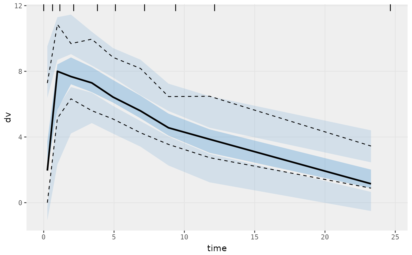
vpcPlot(fit)
#>  
#>  


# }